The Transformer, block by block
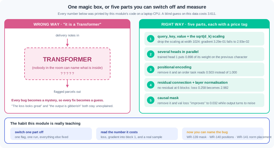
Bhargavi tests AI features at a logistics firm in Rourkela. Her team ships a model that reads delivery notes and flags late parcels. In a design review her lead asks her to draw the model on the whiteboard. She draws one big box and writes "Transformer" inside it. Her lead smiles and says the box has five parts, and every bug they filed last month lived inside one of them. Tonight Bhargavi builds those five parts herself, one at a time, on her own laptop.
- Every model in Phase 3 is this architecture. Once you have built the parts yourself, LLM code, RAG code and agent code stop looking like magic and start looking like layers you can name.
- "Explain a Transformer block" is the single most asked deep-learning question in Indian AI interviews, and tonight your answer is a measured table with your own numbers in it.
- The whole module runs on an 8GB laptop with no GPU. The tiny GPT below trains in 34 seconds and writes readable sentences, and every number printed here came from that machine.
Module 2.7 ended with attention worked out by hand on four tokens. That small NumPy function is the seed of this module. A Transformer is that same function, wrapped in four more parts and stacked a few times. Nothing else hides inside the box. Tonight you build each part and measure what it is worth.
There is a wrong way and a right way to hold this idea. The wrong way treats the model as one magic box: text goes in, text comes out, and every fault is a mystery. The right way names five parts — query-key-value attention, several heads, position information, the residual-and-norm wrapper, and the causal mask. Each part has a job you can switch off and measure. Take the residual links out of a six-block model and its loss stops at 2.982 against 0.258, which is the gap between a working model and noise.
Self-attention — every position reading every other position in the same sequence — begins with three small projections. Each token makes a query, a key and a value. The query says what I am looking for. The key says what I offer to anyone who asks. The value says what I hand over when I am picked.
Those three come from three learned matrices, and 2.7's single set of vectors was the beginner's version. In the toy below, the word "late" carries a problem, so its query asks for an item and a place. The words "parcel" and "warehouse" answer with matching keys, and each takes 0.425 of the weight. The word "late" then leaves the layer holding an item number of 0.851 and a place number of 0.851, both of which were zero on the way in. One layer turned a lone adjective into a fact about a parcel at a warehouse.
Scores are dot products, so they grow with the width of the vectors. At a key width of 1024 the raw scores spread out by about 31, and softmax handed 0.860 of the weight to a single key. A near-certain choice leaves almost no gradient, measured here as 2.93e-02 against 3.29e-01. Dividing every score by the square root of the key width undoes that growth. The same draw then spreads its weight as 0.244, 0.231, 0.176 and so on, and learning has something to work with.
Multi-head attention — several attention patterns computed side by side and then joined — lets one layer hold more than one habit. Each head gets a slice of the width, so two heads cost about what one wide head costs. In the trained model below, head 1 puts 0.898 of its average weight on the character right before it. Head 0 spreads its weight over the last few characters instead. Two heads, two habits, one layer.
Attention by itself has no sense of order. Shuffle the rows of the input and every output row moves with its token, otherwise unchanged. The measured gap between the two runs was 5.96e-08, which is rounding noise. Positional encoding — a vector added to each token that says where it sits in the line — repairs this. On a task where order alone decides the label, the same model scored 0.503 without positions and 1.000 with them.
Around attention sit three more pieces, and together they make a block. A residual connection — adding a layer's input to its own output — gives the gradient a short road back to the start. Layer normalisation — rescaling each token's vector to a steady mean and spread — keeps the numbers in a safe range as depth grows. A feed-forward network then works on each position on its own, four times wider in the middle. Norm, attention, add, norm, feed-forward, add: that is the whole block.
These parts are not decoration, and the table below prices them. At six blocks, dropping the residual links moved the gradient reaching block 1 from 5.951e-02 to 1.785e-07. The loss stayed at 2.982, close to the 3.611 that a blind guess costs on this data. Layer normalisation looks harmless at a gentle learning rate. Raise the rate to 0.01 and the run without norm reads 1.434 while the pre-norm run reads 0.256.
A GPT is this block with one more rule. A causal mask — a matrix that forbids each position from reading anything later than itself — turns the stack into a next-token predictor. Position 3 may read positions 0 to 3, and the rest of the row is set to minus infinity before softmax. Take the mask away and the model reads the very character it is meant to predict, so its loss falls to 0.032 and its output turns to gibberish. That is 1.7's leakage, wearing an architecture costume.
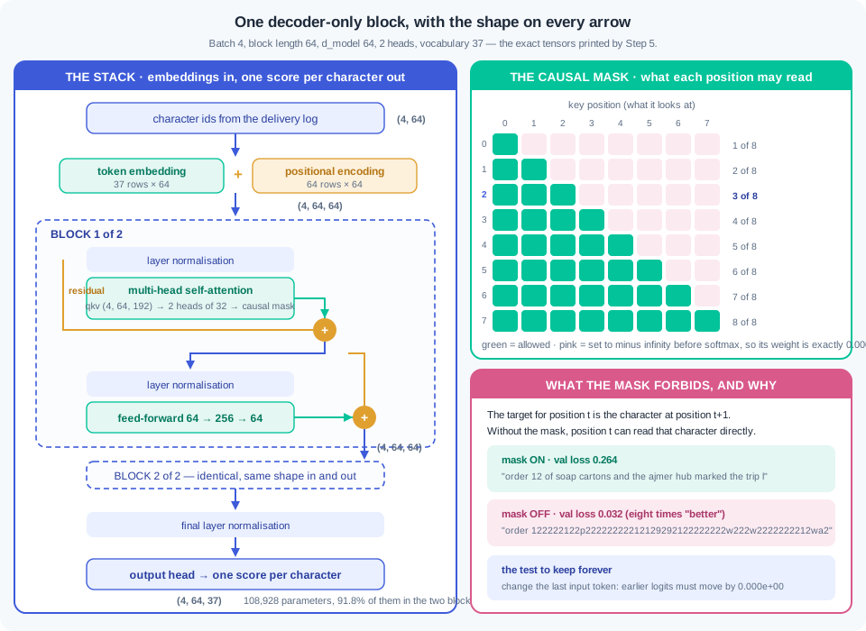
Counting parameters turns Phase 3's cost lessons into arithmetic. The tiny model below holds 108,928 numbers, and 91.8 percent of them sit in its two blocks. The same formula at width 4096 and 32 layers gives 6.7 billion numbers, about 13.4 GB in half precision. Attention score matrices grow with the square of the context, so 4096 tokens need 68.7 GB of them and 32,768 tokens need 4398 GB. Module 3.1 described this loop from the outside; this module is the same loop from the inside, and the price now has a formula.
Work inside ai-lab with torch and numpy. One-time setup: pip install torch==2.9.* numpy==2.5.* — the CPU build is all this course needs. Nothing is downloaded: the corpus in steps 5 to 7 is written by code, so the whole module runs offline on an 8GB laptop with no GPU. Timings come from a plain CPU laptop with four threads. Every seed is fixed, so losses and accuracies below should land within about 1% of your screen — seeded torch runs vary slightly across builds — while vocabulary sizes, parameter counts and shapes should match exactly; wall-clock seconds will differ.
If your numbers are close but not identical, triage in a fixed order before touching your code. Everything off by a little — every value drifting in the last decimal or two — points at a library version: run pip show torch, compare it with the pinned install line above, and match the pin, because the printed numbers were produced on that version. One number wildly off while the rest agree points at stale state: restart from a fresh kernel or a fresh python and run the file top to bottom, since seeded draws only reproduce when they happen in the same order from a clean start. Only when both checks pass and the numbers still disagree should you suspect your own logic — diff your script line by line against the printed code.
Step 1 — query, key and value, printed as matrices. Save this as transformer_bits.py; later steps import it:
import numpy as np, torch, torch.nn as nn

torch.set_num_threads(4)
np.set_printoptions(precision=3, suppress=True)

TOKENS = ["parcel", "left", "warehouse", "late"]
AXES = ["item", "place", "time", "problem"]

# One row per token: 2.7's hand-made meanings, four numbers each.
E = np.array([[2.0, 0.0, 0.0, 0.0],      # parcel     -> an item
              [0.0, 0.0, 1.5, 0.0],      # left       -> a time word
              [0.0, 2.0, 0.0, 0.0],      # warehouse  -> a place
              [0.0, 0.0, 0.5, 2.0]])     # late       -> a problem, a little time-ish

D_MODEL = E.shape[1]

# In a real Transformer these three come out of training. Here they are hand-set
# so the printed numbers can be read.
WQ = np.array([[0.0, 0.0, 0.0, 0.0],
               [0.0, 0.0, 0.0, 0.0],
               [0.0, 0.0, 1.0, 0.0],     # a time word asks about time
               [1.0, 1.0, 0.0, 0.0]])    # a problem word asks: which item, which place
WK = np.eye(4)                            # key = what I openly offer
WV = np.diag([1.0, 1.0, 0.0, 1.0])        # value = what I hand over (time axis dropped)


def softmax(x, axis=-1):
    e = np.exp(x - x.max(axis=axis, keepdims=True))
    return e / e.sum(axis=axis, keepdims=True)


def show(name, mat, rows=TOKENS, cols=None):
    print(f"{name}")
    if cols:
        print(f"{'':<11s}" + "".join(f"{c:>11s}" for c in cols))
    for r, row in zip(rows, mat):
        print(f"  {r:<9s}" + "".join(f"{v:11.3f}" for v in row))


# ---- step1_qkv.py starts here ----
Q, K, V = E @ WQ, E @ WK, E @ WV
show("Q = E @ Wq   (what am I looking for)", Q, cols=AXES)
show("K = E @ Wk   (what do I offer)", K, cols=AXES)
show("V = E @ Wv   (what do I carry)", V, cols=AXES)

d_k = Q.shape[1]
scores = Q @ K.T / np.sqrt(d_k)
show(f"scores divided by sqrt(d_k) = {np.sqrt(d_k):.3f}", scores, cols=TOKENS)
W = softmax(scores)
show("attention weights (each row adds to 1.000)", W, cols=TOKENS)
out = W @ V
show("output = weights @ V", out, cols=AXES)

i = TOKENS.index("late")
for j, t in enumerate(TOKENS):
    print(f"  {W[i, j]:.3f} of its new meaning comes from '{t}'")
print(f"  item number {E[i, 0]:+.3f} -> {out[i, 0]:+.3f}"
      f"   place number {E[i, 1]:+.3f} -> {out[i, 1]:+.3f}")

t = torch.nn.functional.scaled_dot_product_attention(
    torch.tensor(Q), torch.tensor(K), torch.tensor(V)).numpy()
print(f"largest gap against torch's own attention: {np.abs(t - out).max():.2e}")
Output:
Q = E @ Wq   (what am I looking for)
                  item      place       time    problem
  parcel         0.000      0.000      0.000      0.000
  left           0.000      0.000      1.500      0.000
  warehouse      0.000      0.000      0.000      0.000
  late           2.000      2.000      0.500      0.000
K = E @ Wk   (what do I offer)
                  item      place       time    problem
  parcel         2.000      0.000      0.000      0.000
  left           0.000      0.000      1.500      0.000
  warehouse      0.000      2.000      0.000      0.000
  late           0.000      0.000      0.500      2.000
V = E @ Wv   (what do I carry)
                  item      place       time    problem
  parcel         2.000      0.000      0.000      0.000
  left           0.000      0.000      0.000      0.000
  warehouse      0.000      2.000      0.000      0.000
  late           0.000      0.000      0.000      2.000
scores divided by sqrt(d_k) = 2.000
                parcel       left  warehouse       late
  parcel         0.000      0.000      0.000      0.000
  left           0.000      1.125      0.000      0.375
  warehouse      0.000      0.000      0.000      0.000
  late           2.000      0.375      2.000      0.125
attention weights (each row adds to 1.000)
                parcel       left  warehouse       late
  parcel         0.250      0.250      0.250      0.250
  left           0.153      0.471      0.153      0.223
  warehouse      0.250      0.250      0.250      0.250
  late           0.425      0.084      0.425      0.065
output = weights @ V
                  item      place       time    problem
  parcel         0.500      0.500      0.000      0.500
  left           0.306      0.306      0.000      0.445
  warehouse      0.500      0.500      0.000      0.500
  late           0.851      0.851      0.000      0.131
  0.425 of its new meaning comes from 'parcel'
  0.084 of its new meaning comes from 'left'
  0.425 of its new meaning comes from 'warehouse'
  0.065 of its new meaning comes from 'late'
  item number +0.000 -> +0.851   place number +0.000 -> +0.851
largest gap against torch's own attention: 8.33e-17
Read the three projections first, because they are the whole idea. Wq is almost empty: only a token with something on the "problem" axis produces a query, which is why the rows for parcel and warehouse are all zeros while late asks [2, 2, 0.5, 0] — "which item, and which place". Wk is the identity here, so a key is what the token openly offers, and Wv drops the time axis, so a value is a smaller thing than a meaning. Now the weights. The rows for parcel and warehouse are flat at 0.250 each, because a token with a zero query has nothing to ask and softmax over four zeros is uniform — a real model learns to avoid this, and an untrained one starts here. The late row is the interesting one: 0.425 on parcel, 0.425 on warehouse, 0.084 and 0.065 on the rest. Read the output row for late last: it entered with [0, 0, 0.5, 2] and leaves with an item number of 0.851 and a place number of 0.851, so a lone complaint word now carries which parcel and which warehouse. The gap of 8.33e-17 against torch.nn.functional.scaled_dot_product_attention says your arithmetic is the arithmetic every Transformer runs.
Step 2 — why the square root is there. Save as step2_scaling.py. One query against eight keys, at five widths, averaged over 400 random draws:
import torch

torch.manual_seed(0)
T, TRIALS = 8, 400


def measure(d_k, scale):
    """Mean largest weight, mean entropy, mean gradient norm into the scores."""
    big, ent, gnorm = [], [], []
    for _ in range(TRIALS):
        q, K = torch.randn(d_k), torch.randn(T, d_k)
        s = (K @ q) / (d_k ** 0.5 if scale else 1.0)
        s.requires_grad_()
        p = torch.softmax(s, -1)
        big.append(float(p.max().detach()))
        ent.append(float(-(p * p.clamp_min(1e-12).log()).sum().detach()))
        (p @ torch.randn(T)).backward()          # any downstream use of the weights
        gnorm.append(float(s.grad.norm()))
    n = len(big)
    return sum(big) / n, sum(ent) / n, sum(gnorm) / n


print(f"Entropy of a flat 8-way choice = {torch.log(torch.tensor(8.0)):.3f} nats\n")
print(f"{'d_k':>6s} {'score std':>10s} | {'NO scaling':>26s} | {'WITH /sqrt(d_k)':>26s}")
print(f"{'':>6s} {'':>10s} | {'max w':>8s} {'entropy':>8s} {'grad':>8s}"
      f" | {'max w':>8s} {'entropy':>8s} {'grad':>8s}")
for d_k in (4, 16, 64, 256, 1024):
    torch.manual_seed(1)
    raw = torch.stack([torch.randn(T, d_k) @ torch.randn(d_k) for _ in range(TRIALS)])
    a, b = measure(d_k, False), measure(d_k, True)
    print(f"{d_k:6d} {float(raw.std()):10.2f} | {a[0]:8.3f} {a[1]:8.3f} {a[2]:8.2e}"
          f" | {b[0]:8.3f} {b[1]:8.3f} {b[2]:8.2e}")

torch.manual_seed(3)
q, K = torch.randn(1024), torch.randn(8, 1024)
raw = K @ q
print("\n  raw scores      :", " ".join(f"{v:+8.2f}" for v in raw))
print("  softmax(raw)    :", " ".join(f"{v:8.3f}" for v in torch.softmax(raw, -1)))
print("  softmax(raw/32) :", " ".join(f"{v:8.3f}" for v in torch.softmax(raw / 32.0, -1)))
Output:
Entropy of a flat 8-way choice = 2.079 nats

   d_k  score std |                 NO scaling |            WITH /sqrt(d_k)
                  |    max w  entropy     grad |    max w  entropy     grad
     4       1.95 |    0.528    1.284 2.99e-01 |    0.332    1.768 3.24e-01
    16       3.90 |    0.769    0.617 2.16e-01 |    0.349    1.739 3.32e-01
    64       8.02 |    0.873    0.320 1.24e-01 |    0.359    1.725 3.34e-01
   256      16.03 |    0.928    0.172 7.68e-02 |    0.364    1.726 3.34e-01
  1024      31.43 |    0.974    0.062 2.93e-02 |    0.363    1.717 3.29e-01

  raw scores      :   -17.46   +19.16   +44.54   +46.36   +35.88   +22.67   +12.09   -55.29
  softmax(raw)    :    0.000    0.000    0.140    0.860    0.000    0.000    0.000    0.000
  softmax(raw/32) :    0.033    0.104    0.231    0.244    0.176    0.117    0.084    0.010
The second column is the cause of everything else. A dot product of two random vectors of width d_k has a spread that grows like the square root of d_k: 1.95 at width 4, 8.02 at width 64, 31.43 at width 1024. Softmax cares about differences between scores, so a spread of 31 means one key wins outright. Watch the "no scaling" group: the largest weight climbs 0.528, 0.769, 0.873, 0.928, 0.974, and entropy falls from 1.284 nats to 0.062 against a flat maximum of 2.079. That is a layer that has made up its mind before training starts. The gradient column is the part that hurts, because a saturated softmax is flat: the gradient norm reaching the scores falls from 2.99e-01 to 2.93e-02, so ten times less signal reaches Wq and Wk. Now the scaled group: max weight sits near 0.36 and entropy near 1.72 at every width, and the gradient holds at about 3.3e-01 from width 4 to width 1024. The single draw at the bottom makes it concrete — raw scores of +44.54 and +46.36 become 0.140 and 0.860, and the same scores divided by 32 become 0.231 and 0.244. The square root of the key width is not decoration; it is what keeps the layer trainable as models get wide.
Step 3 — several heads, several habits. Save as step3_heads.py. Two hand-set heads on one eight-token line, so the printed patterns can be read:
import torch, torch.nn as nn

WORDS = ["parcel", "for", "kirana", "shop", "reached", "warehouse", "late", "again"]
#                 item  for  shop  action place problem
E = torch.tensor([[2., 0., 0., 0., 0., 0.],   # parcel
                  [0., 2., 0., 0., 0., 0.],   # for
                  [0., 0., 1., 0., 0., 0.],   # kirana
                  [0., 0., 2., 0., 0., 0.],   # shop
                  [0., 0., 0., 2., 0., 0.],   # reached
                  [0., 0., 0., 0., 2., 0.],   # warehouse
                  [0., 0., 0., 0., 0., 2.],   # late
                  [0., 0., 0., 0., 0., .5]])  # again
D, H = 6, 2
DH = D // H

Wq, bq = torch.zeros(D, D), torch.zeros(D)
Wk, bk = torch.zeros(D, D), torch.zeros(D)
Wv = torch.eye(D)
# head 0 uses slots 0..2, head 1 uses slots 3..5
Wq[5, 0] = Wq[5, 1] = 1.0     # HEAD 0: a problem word asks for an item and a place
Wk[0, 0] = 1.0
Wk[4, 1] = 1.0
bq[3] = 2.0                    # HEAD 1: every token asks the same thing, from the bias
Wk[3, 3] = 1.0                 #         and only the action word answers


def heads(X):
    Q, K, V = X @ Wq + bq, X @ Wk + bk, X @ Wv
    T = X.shape[0]
    Qh, Kh, Vh = (t.view(T, H, DH).transpose(0, 1) for t in (Q, K, V))
    W = torch.softmax(Qh @ Kh.transpose(-2, -1) / DH ** 0.5, -1)
    O = W @ Vh                                    # (H, T, DH)
    return W, O.transpose(0, 1).reshape(T, D)     # concatenate the heads back


W, cat = heads(E)
print(f"d_model={D}, heads={H}, d_head={DH}")
print(f"shapes: X {tuple(E.shape)} -> per-head weights {tuple(W.shape)}"
      f" -> concat {tuple(cat.shape)}")
for h in range(H):
    print(f"\nHEAD {h}")
    print(f"{'':<11s}" + "".join(f"{w:>10s}" for w in WORDS))
    for w, row in zip(WORDS, W[h]):
        print(f"  {w:<9s}" + "".join(f"{v:10.3f}" for v in row))

mha = nn.MultiheadAttention(D, H, bias=True, batch_first=True)
with torch.no_grad():
    mha.in_proj_weight.copy_(torch.cat([Wq.T, Wk.T, Wv.T], 0))
    mha.in_proj_bias.copy_(torch.cat([bq, bk, torch.zeros(D)]))
    mha.out_proj.weight.copy_(torch.eye(D)); mha.out_proj.bias.zero_()
    ref, _ = mha(E[None], E[None], E[None])
print(f"\ngap against torch's nn.MultiheadAttention: {float((ref[0] - cat).abs().max()):.2e}")
Output:
d_model=6, heads=2, d_head=3
shapes: X (8, 6) -> per-head weights (2, 8, 8) -> concat (8, 6)

HEAD 0
               parcel       for    kirana      shop   reached warehouse      late     again
  parcel        0.125     0.125     0.125     0.125     0.125     0.125     0.125     0.125
  for           0.125     0.125     0.125     0.125     0.125     0.125     0.125     0.125
  kirana        0.125     0.125     0.125     0.125     0.125     0.125     0.125     0.125
  shop          0.125     0.125     0.125     0.125     0.125     0.125     0.125     0.125
  reached       0.125     0.125     0.125     0.125     0.125     0.125     0.125     0.125
  warehouse     0.125     0.125     0.125     0.125     0.125     0.125     0.125     0.125
  late          0.385     0.038     0.038     0.038     0.038     0.385     0.038     0.038
  again         0.186     0.105     0.105     0.105     0.105     0.186     0.105     0.105

HEAD 1
               parcel       for    kirana      shop   reached warehouse      late     again
  parcel        0.059     0.059     0.059     0.059     0.590     0.059     0.059     0.059
  for           0.059     0.059     0.059     0.059     0.590     0.059     0.059     0.059
  kirana        0.059     0.059     0.059     0.059     0.590     0.059     0.059     0.059
  shop          0.059     0.059     0.059     0.059     0.590     0.059     0.059     0.059
  reached       0.059     0.059     0.059     0.059     0.590     0.059     0.059     0.059
  warehouse     0.059     0.059     0.059     0.059     0.590     0.059     0.059     0.059
  late          0.059     0.059     0.059     0.059     0.590     0.059     0.059     0.059
  again         0.059     0.059     0.059     0.059     0.590     0.059     0.059     0.059

gap against torch's nn.MultiheadAttention: 0.00e+00
Two heads, and they are doing different jobs on the same eight words. Head 0 is a complaint-resolver: only late and again sit on the "problem" axis, so only their rows depart from the flat 0.125, and the late row puts 0.385 on parcel and 0.385 on warehouse — which item, at which place. Note the again row: it holds 0.5 on the problem axis instead of 2.0, so it asks the same question more weakly and gets 0.186 and 0.186. Strength of the query, not the identity of the token, sets how sharp a row is. Head 1 is a completely different animal: its query comes from a bias, so every single row is identical and every token puts 0.590 on reached, the one word carrying the action axis. That is a "find the verb" head, and heads like it appear in real trained models under names like "previous token head" and "punctuation head". The two heads use slots 0 to 2 and slots 3 to 5 of the same six numbers, so they cost together what one head of width 6 would cost. The final 0.00e+00 against nn.MultiheadAttention proves the reshape-transpose-softmax-reshape dance is exactly what PyTorch does, once you load the same weights into it.
Step 4 — proving attention is blind to order, then fixing it. Save as step4_positions.py:
import time, torch, torch.nn as nn

torch.set_num_threads(4)
torch.manual_seed(0)
T, D = 8, 16
X = torch.randn(T, D)
attn = nn.MultiheadAttention(D, 2, batch_first=True); attn.eval()


@torch.no_grad()
def run(x):
    return attn(x[None], x[None], x[None])[0][0]


perm = torch.tensor([4, 0, 7, 2, 6, 1, 5, 3])
a, b = run(X), run(X[perm])
print(f"gap between run(X)[perm] and run(X[perm]): {float((a[perm] - b).abs().max()):.2e}")


def sinusoid(T, D):
    pos = torch.arange(T).float()[:, None]
    i = torch.arange(0, D, 2).float()[None, :]
    ang = pos / (10000 ** (i / D))
    P = torch.zeros(T, D)
    P[:, 0::2], P[:, 1::2] = torch.sin(ang), torch.cos(ang)
    return P


P = sinusoid(T, D)
print(f"positional encoding, first 6 of {D} columns:")
for t in range(T):
    print(f"  pos {t}: " + " ".join(f"{v:+.3f}" for v in P[t, :6]))
a2, b2 = run(X + P), run(X[perm] + P)
print(f"with positions added, the same gap: {float((a2[perm] - b2).abs().max()):.3f}")

VOC, LEN = 8, 12                      # 0 = token A, 1 = token B, 2..7 = filler


def order_task(n, seed):
    """One A and one B among filler. Label = 1 when A comes before B."""
    g = torch.Generator().manual_seed(seed)
    x = torch.randint(2, VOC, (n, LEN), generator=g)
    y = torch.zeros(n)
    for r in range(n):
        i, j = torch.randperm(LEN, generator=g)[:2].tolist()
        x[r, i], x[r, j] = 0, 1
        y[r] = float(i < j)
    return x, y


class Tiny(nn.Module):
    def __init__(self, use_pos):
        super().__init__()
        self.emb = nn.Embedding(VOC, 32)
        self.pos = nn.Parameter(sinusoid(LEN, 32), requires_grad=False)
        self.use_pos = use_pos
        self.att = nn.MultiheadAttention(32, 2, batch_first=True)
        self.head = nn.Linear(32, 1)

    def forward(self, x):
        h = self.emb(x)
        if self.use_pos:
            h = h + self.pos
        h, _ = self.att(h, h, h)
        return self.head(h.mean(1)).squeeze(-1)


Xtr, ytr = order_task(4000, 21)
Xte, yte = order_task(1000, 22)
print(f"\n{'model':<26s} {'params':>8s} {'train s':>8s} {'train acc':>10s} {'test acc':>9s}")
for label, use_pos in (("attention, no positions", False), ("attention + positions", True)):
    torch.manual_seed(7)
    net = Tiny(use_pos)
    opt = torch.optim.Adam(net.parameters(), lr=0.01)
    g = torch.Generator().manual_seed(7)
    t0 = time.perf_counter()
    for _ in range(30):
        for i in torch.randperm(len(Xtr), generator=g).split(64):
            opt.zero_grad()
            nn.functional.binary_cross_entropy_with_logits(net(Xtr[i]), ytr[i]).backward()
            opt.step()
    dt = time.perf_counter() - t0
    with torch.no_grad():
        tr = float(((net(Xtr) > 0).float() == ytr).float().mean())
        te = float(((net(Xte) > 0).float() == yte).float().mean())
    n_par = sum(p.numel() for p in net.parameters() if p.requires_grad)
    print(f"{label:<26s} {n_par:8,d} {dt:8.1f} {tr:10.3f} {te:9.3f}")
Output:
gap between run(X)[perm] and run(X[perm]): 5.96e-08
positional encoding, first 6 of 16 columns:
  pos 0: +0.000 +1.000 +0.000 +1.000 +0.000 +1.000
  pos 1: +0.841 +0.540 +0.311 +0.950 +0.100 +0.995
  pos 2: +0.909 -0.416 +0.591 +0.807 +0.199 +0.980
  pos 3: +0.141 -0.990 +0.813 +0.583 +0.296 +0.955
  pos 4: -0.757 -0.654 +0.954 +0.301 +0.389 +0.921
  pos 5: -0.959 +0.284 +1.000 -0.010 +0.479 +0.878
  pos 6: -0.279 +0.960 +0.947 -0.321 +0.565 +0.825
  pos 7: +0.657 +0.754 +0.800 -0.599 +0.644 +0.765
with positions added, the same gap: 0.264

model                        params  train s  train acc  test acc
attention, no positions       4,513      1.9      0.543     0.503
attention + positions         4,513      1.9      1.000     1.000
The first line is a proof, not a demonstration. Feed the eight token vectors in a shuffled order and the layer returns the same eight output vectors, shuffled the same way — the largest gap is 5.96e-08, which is float32 rounding. An attention layer is a set-reader: to it, "parcel reached warehouse late" and "late warehouse reached parcel" are the same input. Look at the positional encoding table and note what makes it usable: every row is different, no row repeats within the block, and neighbouring rows are similar, so position 3 looks more like position 4 than like position 7. Add it and the same shuffle now moves the outputs by 0.264, which means the layer can finally tell the two orders apart. The training table prices the fix. Both models have exactly 4,513 trainable parameters and both take 1.9 seconds, but the one without positions reads 0.503 on held-back rows — a coin toss on a task where order is the only signal — while the one with positions reads 1.000. Its 0.543 training accuracy is the honest tell: it did not overfit, it never learned anything, because the information was not in its input at all. WR-140 is what this looks like when nobody runs the test.
Step 5 — the whole block, then take pieces out. Save corpus.py and tiny_gpt.py first; every remaining step imports them:
# ---------------- corpus.py : an Indian-context corpus written by code ----------------
import numpy as np, torch

CITIES = ["rourkela", "bhilai", "nellore", "ajmer", "thrissur", "sangli"]
GOODS = ["rice bags", "soap cartons", "tea packets", "oil tins", "salt packs",
         "biscuit boxes"]
SHOPS = ["kirana shop", "medical store", "sweet shop", "hardware store"]
DRIVERS = ["ravi", "imran", "joseph", "gopal", "tara", "hemant"]
STATES = ["picked up", "loaded", "in transit", "delivered", "returned"]


def build_corpus(n_lines=6000, seed=5):
    rng = np.random.default_rng(seed)
    out = []
    for _ in range(n_lines):
        c1, c2 = rng.choice(CITIES, 2, replace=False)
        g, s, d = rng.choice(GOODS), rng.choice(SHOPS), rng.choice(DRIVERS)
        st, box = rng.choice(STATES), rng.integers(2, 40)
        hh, mm = rng.integers(6, 21), rng.choice([0, 15, 30, 45])
        pick = rng.random()
        if pick < 0.34:
            out.append(f"{d} carried {box} {g} from the {c1} hub to the "
                       f"{s} in {c2} at {hh:02d}:{mm:02d} and the parcel was {st} .")
        elif pick < 0.67:
            out.append(f"the {s} in {c2} ordered {box} {g} and the {c1} hub "
                       f"marked the trip {st} at {hh:02d}:{mm:02d} .")
        else:
            out.append(f"order {box} of {g} for the {s} in {c2} left the {c1} "
                       f"hub at {hh:02d}:{mm:02d} with {d} and was {st} .")
    return "\n".join(out) + "\n"


def make_dataset(text, val_frac=0.1):
    chars = sorted(set(text))
    stoi = {c: i for i, c in enumerate(chars)}
    data = torch.tensor([stoi[c] for c in text], dtype=torch.long)
    n = int(len(data) * (1 - val_frac))
    return chars, stoi, data[:n], data[n:]


def get_batch(data, block, batch, gen):
    ix = torch.randint(len(data) - block - 1, (batch,), generator=gen)
    x = torch.stack([data[i:i + block] for i in ix])
    y = torch.stack([data[i + 1:i + 1 + block] for i in ix])
    return x, y


# ---------------- tiny_gpt.py : the model, with every part switchable ----------------
import torch.nn as nn, torch.nn.functional as F

torch.set_num_threads(4)


class SelfAttention(nn.Module):
    def __init__(self, d_model, n_head, causal=True):
        super().__init__()
        self.h, self.dh, self.causal = n_head, d_model // n_head, causal
        self.qkv = nn.Linear(d_model, 3 * d_model)
        self.proj = nn.Linear(d_model, d_model)

    def forward(self, x, keep=False):
        B, T, D = x.shape
        q, k, v = self.qkv(x).split(D, dim=2)
        q, k, v = (t.view(B, T, self.h, self.dh).transpose(1, 2) for t in (q, k, v))
        s = q @ k.transpose(-2, -1) / self.dh ** 0.5
        if self.causal:
            s = s.masked_fill(torch.triu(torch.ones(T, T, dtype=torch.bool), 1),
                              float("-inf"))
        w = s.softmax(-1)
        if keep:
            self.last_weights = w.detach()
        return self.proj((w @ v).transpose(1, 2).reshape(B, T, D))


class Block(nn.Module):
    """attention -> residual+norm -> feed-forward -> residual+norm."""

    def __init__(self, d_model, n_head, causal=True, residual=True, norm=True,
                 prenorm=True):
        super().__init__()
        self.att = SelfAttention(d_model, n_head, causal)
        self.ff = nn.Sequential(nn.Linear(d_model, 4 * d_model), nn.GELU(),
                                nn.Linear(4 * d_model, d_model))
        self.n1 = nn.LayerNorm(d_model) if norm else nn.Identity()
        self.n2 = nn.LayerNorm(d_model) if norm else nn.Identity()
        self.residual, self.prenorm = residual, prenorm

    def forward(self, x, keep=False):
        if self.prenorm:                       # norm INSIDE the branch
            a = self.att(self.n1(x), keep)
            x = x + a if self.residual else a
            f = self.ff(self.n2(x))
            return x + f if self.residual else f
        a = self.att(x, keep)                  # norm AFTER the add
        x = self.n1(x + a if self.residual else a)
        f = self.ff(x)
        return self.n2(x + f if self.residual else f)


class TinyGPT(nn.Module):
    def __init__(self, vocab, block=64, d_model=64, n_head=2, n_layer=2,
                 causal=True, residual=True, norm=True, positions=True, prenorm=True):
        super().__init__()
        self.block, self.positions = block, positions
        self.tok = nn.Embedding(vocab, d_model)
        self.pos = nn.Embedding(block, d_model)
        self.blocks = nn.ModuleList([Block(d_model, n_head, causal, residual, norm,
                                           prenorm) for _ in range(n_layer)])
        self.nf = nn.LayerNorm(d_model) if norm else nn.Identity()
        self.head = nn.Linear(d_model, vocab, bias=False)

    def forward(self, idx, targets=None, keep=False):
        B, T = idx.shape
        x = self.tok(idx)
        if self.positions:
            x = x + self.pos(torch.arange(T))
        for b in self.blocks:
            x = b(x, keep)
        logits = self.head(self.nf(x))
        if targets is None:
            return logits, None
        return logits, F.cross_entropy(logits.view(B * T, -1), targets.reshape(B * T))

    @torch.no_grad()
    def generate(self, idx, n, temperature=0.8, gen=None):
        for _ in range(n):
            logits, _ = self(idx[:, -self.block:])
            probs = (logits[:, -1, :] / temperature).softmax(-1)
            idx = torch.cat([idx, torch.multinomial(probs, 1, generator=gen)], 1)
        return idx


def n_params(model):
    return sum(p.numel() for p in model.parameters())


# ---------------- step5_block.py : shapes, then the ablations ----------------
import math, time
from corpus import build_corpus, make_dataset, get_batch
from tiny_gpt import TinyGPT

text = build_corpus()
chars, stoi, train, val = make_dataset(text)
V, BLOCK, STEPS = len(chars), 64, 300
print(f"corpus {len(text):,d} characters, vocabulary {V}")
print(f"a flat guess over {V} characters costs ln({V}) = {math.log(V):.3f}\n")

x, y = get_batch(train, BLOCK, 4, torch.Generator().manual_seed(0))
probe = TinyGPT(V, BLOCK, 64, 2, 2)
h = probe.tok(x) + probe.pos(torch.arange(BLOCK))
print("shapes through one block, batch 4:")
print(f"  token ids            {tuple(x.shape)}")
print(f"  after embed+position {tuple(h.shape)}")
print(f"  qkv projection       {tuple(probe.blocks[0].att.qkv(h).shape)}")
print(f"  after block 1        {tuple(probe.blocks[0](h).shape)}")
print(f"  logits               {tuple(probe(x)[0].shape)}\n")


def run(layers, **kw):
    torch.manual_seed(7)
    m = TinyGPT(V, BLOCK, 64, 2, layers, **kw)
    opt = torch.optim.AdamW(m.parameters(), lr=3e-3)
    g = torch.Generator().manual_seed(7)
    t0, g1 = time.perf_counter(), None
    for s in range(STEPS):
        xb, yb = get_batch(train, BLOCK, 32, g)
        _, loss = m(xb, yb)
        opt.zero_grad(); loss.backward()
        if s == STEPS - 1:
            g1 = float(m.blocks[0].att.qkv.weight.grad.norm())
        opt.step()
    dt = time.perf_counter() - t0
    m.eval()
    with torch.no_grad():
        vg = torch.Generator().manual_seed(3)
        vl = sum(float(m(*get_batch(val, BLOCK, 32, vg))[1]) for _ in range(10)) / 10
    return dt, float(loss.detach()), vl, g1


print(f"{'variant':<34s} {'depth':>5s} {'s':>6s} {'train loss':>11s}"
      f" {'val loss':>9s} {'grad into block 1':>18s}")
for layers in (2, 6):
    for label, kw in (("full block", {}),
                      ("no residual connections", {"residual": False}),
                      ("no layer normalisation", {"norm": False}),
                      ("no residual and no norm", {"residual": False, "norm": False})):
        dt, tl, vl, g1 = run(layers, **kw)
        print(f"{label:<34s} {layers:5d} {dt:6.1f} {tl:11.3f} {vl:9.3f} {g1:18.3e}")

print(f"\nsix blocks, same {STEPS} steps, one knob changed: where the norm sits")
print(f"{'learning rate':>14s} {'pre-norm':>12s} {'post-norm':>12s} {'no norm':>12s}")
for lr in (1e-3, 3e-3, 1e-2, 3e-2):
    row = []
    for kw in ({"prenorm": True}, {"prenorm": False}, {"norm": False}):
        torch.manual_seed(7)
        m = TinyGPT(V, BLOCK, 64, 2, 6, **kw)
        opt = torch.optim.AdamW(m.parameters(), lr=lr)
        g = torch.Generator().manual_seed(7)
        for _ in range(STEPS):
            xb, yb = get_batch(train, BLOCK, 32, g)
            _, loss = m(xb, yb)
            opt.zero_grad(); loss.backward(); opt.step()
        row.append(float(loss.detach()))
    print(f"{lr:14.0e} " + "".join(f"{v:12.4g}" for v in row))
Output:
corpus 680,871 characters, vocabulary 37
a flat guess over 37 characters costs ln(37) = 3.611

shapes through one block, batch 4:
  token ids            (4, 64)
  after embed+position (4, 64, 64)
  qkv projection       (4, 64, 192)
  after block 1        (4, 64, 64)
  logits               (4, 64, 37)

variant                            depth      s  train loss  val loss  grad into block 1
full block                             2    1.9       0.300     0.296          1.295e-01
no residual connections                2    1.8       2.841     2.841          6.191e-02
no layer normalisation                 2    1.7       0.325     0.302          2.391e-01
no residual and no norm                2    1.7       1.978     1.969          7.475e-01
full block                             6    5.3       0.258     0.256          5.951e-02
no residual connections                6    5.2       2.982     2.994          1.785e-07
no layer normalisation                 6    4.9       0.276     0.273          6.879e-02
no residual and no norm                6    4.7       2.981     2.993          1.289e-08

six blocks, same 300 steps, one knob changed: where the norm sits
 learning rate     pre-norm    post-norm      no norm
         1e-03         0.37      0.3656      0.3308
         3e-03       0.2584      0.2598      0.2761
         1e-02       0.2556       2.892       1.434
         3e-02       0.4312       2.981   2.327e+10
Start with the shape trace, because it is the map you will use to read any Transformer code. A batch of 4 lines of 64 characters becomes (4, 64, 64) after the embedding and position are added, the qkv layer widens that to (4, 64, 192) because query, key and value are computed in one matrix multiply and then split three ways, the block returns the same (4, 64, 64) it was given, and the head turns each position into 37 character scores. Every Transformer keeps this shape from the first block to the last; only the width and the number of blocks change. Now the ablation table, and read the depth-6 rows first. Removing the residual links takes the loss from 0.258 to 2.982 — barely below the 3.611 a blind guess costs — and the gradient reaching block 1 collapses from 5.951e-02 to 1.785e-07. That is 2.7's vanishing gradient again, in depth instead of in time, and the residual is the highway that fixes it. At depth 2 the same ablation is far less brutal, 2.841, which tells you the residual is not about attention at all; it is about depth. Layer normalisation looks almost free in this table: 0.276 against 0.258. The last table shows the bill it was quietly paying. At a learning rate of 0.001 all three variants are within 0.04 of each other, at 0.01 the no-norm run reads 1.434 and the post-norm run reads 2.892 while pre-norm reads 0.256, and at 0.03 the no-norm run reaches 2.327e+10. Norm buys you a wide range of usable learning rates, which is why every modern model puts the norm inside the branch before attention, and WR-141 is the version of this you meet at 2 am.
Step 6 — the causal mask, and what happens without it. Save as step6_mask.py:
import math, time, torch
from corpus import build_corpus, make_dataset, get_batch
from tiny_gpt import TinyGPT

text = build_corpus()
chars, stoi, train, val = make_dataset(text)
itos = {i: c for c, i in stoi.items()}
V, BLOCK, STEPS, T = len(chars), 64, 400, 8

mask = torch.triu(torch.ones(T, T, dtype=torch.bool), 1)
print("causal mask for 8 positions: 1 = allowed, . = forbidden")
print("        " + "".join(f"{j:>4d}" for j in range(T)) + "   may look at")
for i in range(T):
    print(f"  pos {i}" + "".join("   ." if mask[i, j] else "   1" for j in range(T))
          + f"   {i + 1} of {T}")

s = torch.randn(T, T).round(decimals=2)
print("\n  raw   :", " ".join(f"{v:+6.2f}" for v in s[2]))
print("  masked:", " ".join(f"{v:+6.2f}" if not mask[2, j] else "  -inf"
                            for j, v in enumerate(s[2])))
print("  weights:", " ".join(f"{v:6.3f}"
      for v in s[2].masked_fill(mask[2], float("-inf")).softmax(-1)))


def train_model(causal):
    torch.manual_seed(7)
    m = TinyGPT(V, BLOCK, 64, 2, 2, causal=causal)
    opt = torch.optim.AdamW(m.parameters(), lr=3e-3)
    g = torch.Generator().manual_seed(7)
    t0 = time.perf_counter()
    for _ in range(STEPS):
        xb, yb = get_batch(train, BLOCK, 32, g)
        _, loss = m(xb, yb)
        opt.zero_grad(); loss.backward(); opt.step()
    dt = time.perf_counter() - t0
    m.eval()
    with torch.no_grad():
        vg = torch.Generator().manual_seed(3)
        vl = sum(float(m(*get_batch(val, BLOCK, 32, vg))[1]) for _ in range(10)) / 10
    return m, float(loss.detach()), vl, dt


print(f"\na flat guess over {V} characters costs ln({V}) = {math.log(V):.3f}")
print(f"{'model':<28s} {'train loss':>11s} {'val loss':>9s} {'s':>6s}")
models = {}
for label, causal in (("causal mask ON (a GPT)", True),
                      ("causal mask OFF (leaking)", False)):
    m, tl, vl, dt = train_model(causal)
    models[label] = m
    print(f"{label:<28s} {tl:11.3f} {vl:9.3f} {dt:6.1f}")

print("\n60 characters generated by each, same seed, prompt 'order 12':")
for label, m in models.items():
    g = torch.Generator().manual_seed(11)
    ctx = torch.tensor([[stoi[c] for c in "order 12"]])
    out = "".join(itos[int(i)] for i in m.generate(ctx, 60, 0.8, g)[0])
    print(f"  {label:<28s} {out.splitlines()[0][:60]!r}")

print("\nthe assertion that catches a leak before training does:")
probe, _ = get_batch(val, 16, 1, torch.Generator().manual_seed(4))
for label, m in models.items():
    with torch.no_grad():
        base, _ = m(probe)
        tampered = probe.clone(); tampered[0, -1] = (int(probe[0, -1]) + 1) % V
        after, _ = m(tampered)
    gap = float((base[0, :-1] - after[0, :-1]).abs().max())
    print(f"  {label:<28s} changing the LAST token moved earlier logits by {gap:.3e}")
Output:
causal mask for 8 positions: 1 = allowed, . = forbidden
           0   1   2   3   4   5   6   7   may look at
  pos 0   1   .   .   .   .   .   .   .   1 of 8
  pos 1   1   1   .   .   .   .   .   .   2 of 8
  pos 2   1   1   1   .   .   .   .   .   3 of 8
  pos 3   1   1   1   1   .   .   .   .   4 of 8
  pos 4   1   1   1   1   1   .   .   .   5 of 8
  pos 5   1   1   1   1   1   1   .   .   6 of 8
  pos 6   1   1   1   1   1   1   1   .   7 of 8
  pos 7   1   1   1   1   1   1   1   1   8 of 8

  raw   :  -1.53  -1.47  +0.44  +0.73  +0.50  -1.07  +1.27  +0.00
  masked:  -1.53  -1.47  +0.44   -inf   -inf   -inf   -inf   -inf
  weights:  0.108  0.115  0.777  0.000  0.000  0.000  0.000  0.000

a flat guess over 37 characters costs ln(37) = 3.611
model                         train loss  val loss      s
causal mask ON (a GPT)             0.273     0.264    2.5
causal mask OFF (leaking)          0.035     0.032    2.5

60 characters generated by each, same seed, prompt 'order 12':
  causal mask ON (a GPT)       'order 12 of soap cartons and the ajmer hub marked the trip l'
  causal mask OFF (leaking)    'order 122222122p22222222212129292122222222w222w2222222212wa2'

the assertion that catches a leak before training does:
  causal mask ON (a GPT)       changing the LAST token moved earlier logits by 0.000e+00
  causal mask OFF (leaking)    changing the LAST token moved earlier logits by 1.265e+01
The mask grid is the definition of a decoder-only model, and it is worth reading one row aloud: position 2 may look at positions 0, 1 and 2, so three of eight, and the rest of its score row becomes minus infinity before the softmax. Minus infinity is the right value because exp(-inf) is exactly 0, so the forbidden weights are 0.000 and the allowed ones still add to 1.000 — the printed row reads 0.108, 0.115, 0.777 and five zeros. Now the table that should scare you. The model without a mask reads a validation loss of 0.032 against 0.264 for the correct model, so on a dashboard it is eight times better. It is not better; the target for position t is the character at position t+1, and without the mask position t can see it. The generation line settles the argument in one look: the masked model writes order 12 of soap cartons and the ajmer hub marked the trip l, and the leaking model writes order 122222122p2222..., because at generation time the future it was trained to peek at does not exist yet. The last two lines are the test you should write once and keep forever: change the final token of an input and check that earlier logits do not move. The correct model moves by exactly 0.000e+00; the leaking one moves by 1.265e+01. WR-139 is this failure with a deadline attached.
Step 7 — a tiny GPT that writes, on a CPU, in under a minute. Save as step7_gpt.py:
import math, os, time, torch
from corpus import build_corpus, make_dataset, get_batch
from tiny_gpt import TinyGPT, n_params

text = build_corpus()
chars, stoi, train, val = make_dataset(text)
itos = {i: c for c, i in stoi.items()}
V, BLOCK, D, H, L = len(chars), 64, 64, 2, 2
STEPS, BATCH, CKPT = 3000, 64, "gpt_ckpt.pt"

torch.manual_seed(7)
model = TinyGPT(V, BLOCK, D, H, L)
opt = torch.optim.AdamW(model.parameters(), lr=3e-3)
g = torch.Generator().manual_seed(7)
print(f"d_model {D}, heads {H}, layers {L}, parameters {n_params(model):,d}")


@torch.no_grad()
def val_loss(m):
    m.eval()
    vg = torch.Generator().manual_seed(3)
    out = sum(float(m(*get_batch(val, BLOCK, 32, vg))[1]) for _ in range(10)) / 10
    m.train()
    return out


def sample(m, n=90, seed=11, prompt="the "):
    m.eval()
    sg = torch.Generator().manual_seed(seed)
    ctx = torch.tensor([[stoi[c] for c in prompt]])
    out = "".join(itos[int(i)] for i in m.generate(ctx, n, 0.8, sg)[0])
    m.train()
    return out.replace("\n", " | ")


start = 0
if os.path.exists(CKPT):                       # resume, per the compute doctrine
    ck = torch.load(CKPT, weights_only=True)
    model.load_state_dict(ck["model"]); opt.load_state_dict(ck["opt"])
    start = ck["step"]
    print(f"resumed from {CKPT} at step {start}")

print(f"{'step':>6s} {'val loss':>9s} {'s':>7s}   90 characters, prompt 'the '")
t0, loss = time.perf_counter(), None
for step in range(start, STEPS + 1):
    if step in (0, 100, 500, 1500, STEPS):
        print(f"{step:6d} {val_loss(model):9.3f} {time.perf_counter() - t0:7.1f}"
              f"   {sample(model)[:74]!r}")
        torch.save({"model": model.state_dict(), "opt": opt.state_dict(),
                    "step": step}, CKPT)
    if step == STEPS:
        break
    xb, yb = get_batch(train, BLOCK, BATCH, g)
    _, loss = model(xb, yb)
    opt.zero_grad(); loss.backward(); opt.step()
print(f"\ntotal training time {time.perf_counter() - t0:.1f} s"
      f" on {torch.get_num_threads()} CPU threads")

print("\nthree longer samples from the finished model:")
for s in (1, 2, 3):
    print(f"  {sample(model, 110, seed=s, prompt='order ')[:100]!r}")

xb, _ = get_batch(val, 14, 1, torch.Generator().manual_seed(2))
line = [itos[int(i)] for i in xb[0]]
with torch.no_grad():
    model.eval(); model(xb, keep=True)
w = model.blocks[0].att.last_weights[0]
print(f"\nlearned attention, layer 1, on {''.join(line)!r}")
for h in range(H):
    print(f"  head {h}:")
    print("        " + "".join(f"{c:>6s}" for c in line))
    for t in range(4, 10):
        print(f"    {line[t]!r:>4s}" + "".join(f"{float(w[h][t][j]):6.2f}"
                                               for j in range(14)))
    prev = sum(float(w[h][t][t - 1]) for t in range(1, 14)) / 13
    self_ = sum(float(w[h][t][t]) for t in range(14)) / 14
    first = sum(float(w[h][t][0]) for t in range(14)) / 14
    print(f"    average weight on: previous {prev:.3f}   itself {self_:.3f}"
          f"   first position {first:.3f}")

groups = {}
for name, p in model.named_parameters():
    key = ("token embedding" if name.startswith("tok") else
           "position embedding" if name.startswith("pos") else
           "output head" if name.startswith("head") else
           "final norm" if name.startswith("nf") else
           "blocks (attention + feed-forward + norms)")
    groups[key] = groups.get(key, 0) + p.numel()
print("\nwhere the parameters live in this model:")
for k, v in groups.items():
    print(f"  {k:<44s} {v:9,d}  {100 * v / n_params(model):5.1f}%")


def count(d, layers, vocab, ctx):
    per_layer = 4 * d * d + 4 * d + 8 * d * d + 5 * d + 4 * d
    return vocab * d + ctx * d + layers * per_layer + 2 * d + vocab * d


print(f"\ncheck: formula {count(D, L, V, BLOCK):,d} vs real {n_params(model):,d}")
print(f"\n{'model':<26s} {'d_model':>8s} {'layers':>7s} {'ctx':>7s} {'parameters':>15s}"
      f" {'fp16 weights':>13s} {'score matrices':>15s}")
for name, d, layers, heads, vocab, ctx in (
        ("this tiny GPT", D, L, H, V, BLOCK),
        ("a 12-layer small model", 768, 12, 12, 50257, 1024),
        ("a 7B-class model", 4096, 32, 32, 32000, 4096),
        ("the same at 32k context", 4096, 32, 32, 32000, 32768)):
    p, scores = count(d, layers, vocab, ctx), layers * heads * ctx * ctx * 4
    print(f"{name:<26s} {d:8d} {layers:7d} {ctx:7d} {p:15,d}"
          f" {p * 2 / 1e9:11.3f}GB {scores / 1e9:13.3f}GB")
Output:
d_model 64, heads 2, layers 2, parameters 108,928
  step  val loss       s   90 characters, prompt 'the '
     0     3.693     0.0   'the ohko.leao | 6ckv0e1198l | jcsps2:k | bg3w35n5lmi lm81 wlfx7o8bbiwu | x'
   100     1.324     1.2   'the bhiturna the a0:115 anal as was and cks thelt 130:4:0 thetord wil the '
   500     0.245     5.8   'the bhilai hub at 08:15 with imran and was loaded . | the kirana shop in t'
  1500     0.230    17.1   'the bhilai hub marked the trip picked up at 17:30 . | order 34 of tea pack'
  3000     0.224    33.9   'the bhilai hub at 08:15 with tara and was delivered . | order 36 of soap c'

total training time 34.0 s on 4 CPU threads

three longer samples from the finished model:
  'order 29 of salt packs for the medical store in ajmer left the nellore hub at 13:00 with imran and w'
  'order 31 of salt packs for the sweet shop in ajmer left the thrissur hub at 16:00 with ravi and was '
  'order 39 of oil tins for the hardware store in bhilai left the bhilai hub at 16:30 with imran and wa'

learned attention, layer 1, on ' hub at 10:15 '
  head 0:
                   h     u     b           a     t           1     0     :     1     5
     ' '  0.01  0.04  0.88  0.07  0.00  0.00  0.00  0.00  0.00  0.00  0.00  0.00  0.00  0.00
     'a'  0.03  0.34  0.13  0.27  0.09  0.15  0.00  0.00  0.00  0.00  0.00  0.00  0.00  0.00
     't'  0.00  0.03  0.02  0.63  0.06  0.23  0.02  0.00  0.00  0.00  0.00  0.00  0.00  0.00
     ' '  0.01  0.03  0.59  0.26  0.01  0.06  0.02  0.01  0.00  0.00  0.00  0.00  0.00  0.00
     '1'  0.01  0.13  0.03  0.21  0.02  0.37  0.12  0.10  0.01  0.00  0.00  0.00  0.00  0.00
     '0'  0.02  0.04  0.09  0.22  0.04  0.22  0.13  0.15  0.03  0.07  0.00  0.00  0.00  0.00
    average weight on: previous 0.177   itself 0.206   first position 0.166
  head 1:
                   h     u     b           a     t           1     0     :     1     5
     ' '  0.00  0.01  0.00  0.99  0.00  0.00  0.00  0.00  0.00  0.00  0.00  0.00  0.00  0.00
     'a'  0.02  0.01  0.02  0.04  0.90  0.02  0.00  0.00  0.00  0.00  0.00  0.00  0.00  0.00
     't'  0.00  0.01  0.02  0.01  0.01  0.94  0.02  0.00  0.00  0.00  0.00  0.00  0.00  0.00
     ' '  0.00  0.00  0.00  0.02  0.00  0.00  0.98  0.00  0.00  0.00  0.00  0.00  0.00  0.00
     '1'  0.00  0.00  0.00  0.01  0.00  0.01  0.00  0.96  0.01  0.00  0.00  0.00  0.00  0.00
     '0'  0.00  0.00  0.00  0.01  0.02  0.01  0.00  0.01  0.92  0.02  0.00  0.00  0.00  0.00
    average weight on: previous 0.898   itself 0.095   first position 0.149

where the parameters live in this model:
  token embedding                                  2,368    2.2%
  position embedding                               4,096    3.8%
  blocks (attention + feed-forward + norms)       99,968   91.8%
  final norm                                         128    0.1%
  output head                                      2,368    2.2%

check: formula 108,928 vs real 108,928

model                       d_model  layers     ctx      parameters  fp16 weights  score matrices
this tiny GPT                    64       2      64         108,928       0.000GB         0.000GB
a 12-layer small model          768      12    1024     163,037,184       0.326GB         0.604GB
a 7B-class model               4096      32    4096   6,723,084,288      13.446GB        68.719GB
the same at 32k context        4096      32   32768   6,840,524,800      13.681GB      4398.047GB
Read the four samples in order, because that progression is the lesson. At step 0 the model is random and produces ohko.leao, 6ckv0e1198l — the right characters in no order at all, and a validation loss of 3.693, slightly worse than the 3.611 a blind guess costs. By step 100, at 1.2 seconds, real words have appeared: the, was, and, plus near-misses like bhiturna and thetord. By step 500 it writes whole clauses that hold together, the bhilai hub at 08:15 with imran and was loaded ., and by step 3000 the three long samples are indistinguishable from corpus lines. Now be honest about what that means. This model has 108,928 parameters and learned one narrow world of six cities, six goods and five states; it writes fluent sentences inside that world and knows nothing outside it, and the flat part of the loss curve from 0.245 to 0.224 says the remaining work is memorising details, not learning grammar. Next, the learned heads, which pay off Step 3's hand-set demonstration: head 1 puts an average of 0.898 of its weight on the character immediately before it, reading 0.99, 0.90, 0.94, 0.98, 0.96 down its rows — nobody designed that, training discovered it. Head 0 is diffuse by comparison, 0.177 on the previous character and 0.206 on itself, spreading over the last few characters like a small word-shaped window. Finally the arithmetic. In this model 91.8 percent of the weights sit in the blocks, which is why "parameters" and "layers times width squared" are almost the same sentence, and the formula matches the real count exactly at 108,928. Read the last table as a bridge to Phase 3: a 7B-class model needs about 13.4 GB of weights in half precision, which is why it will not fit on your laptop, and its attention score matrices need 68.7 GB at 4096 tokens and 4398 GB at 32,768 tokens. That single row is the reason long context costs money, the reason FlashAttention and paged caches exist, and the reason 3.1's context window has a hard edge.
Work inside ai-lab with torch and numpy, and keep transformer_bits.py, corpus.py and tiny_gpt.py in the folder, because the exercises import them. Nothing downloads and nothing needs a GPU. Every seed is fixed, so where a loss or an accuracy is given your output should land within about 1% of it — seeded torch runs vary slightly across builds — while shapes and counts should match exactly; wall-clock seconds will differ with your machine, and that is expected. Exercise 4 is the longest run at roughly 34 seconds of training. If your laptop is much slower, cut STEPS and say so in your comments rather than reporting a number you did not measure. If you want a bigger corpus or a wider model, take it to a Kaggle CPU or GPU session and keep the checkpoint-resume code either way.
Query, key, value, and the square root. Create qkv_lab.py. Part one: rebuild Step 1's four tokens and three projection matrices, then print Q, K, V, the raw score matrix, the scaled score matrix and the weight matrix, and confirm every weight row sums to 1.000. Part two: write four comment sentences that name, for the late row, which token it asks for, which two tokens answer, what number replaced the zero on its item axis, and why the parcel and warehouse rows are flat at 0.250. Part three: change one thing at a time and record the effect in a small table — set WQ to the identity, then set WV to the identity, then multiply all of E by 3 — reporting the late row's largest weight in each case. Part four: reproduce Step 2's scaling table at key widths 4, 16, 64, 256 and 1024, then add two columns of your own: the score standard deviation divided by the square root of the width, and the largest weight when you divide by d_k instead of by its square root. Check: your unscaled table shows the largest weight climbing from 0.528 at width 4 to 0.974 at width 1024 while entropy falls from 1.284 to 0.062, and the scaled columns stay near 0.36 and 1.72 at every width; the gradient column falls from 2.99e-01 to 2.93e-02 unscaled and holds near 3.3e-01 scaled; your new column shows the standard deviation divided by the square root of the width is roughly constant near 1.0, which is the reason the fix works; dividing by d_k instead makes the weights almost uniform, and your comment states that over-flattening costs the layer its ability to choose; and tripling E sharpens the late row, with a comment naming score size, not vocabulary, as the cause.
Heads that disagree, and the permutation test. Create heads_and_positions.py. Part one: reproduce Step 3's two hand-set heads, print both weight matrices, and write three comment sentences describing head 0, describing head 1, and explaining why the again row is softer than the late row. Part two: add a third head of your own design on the same eight tokens — pick a job, set Wq and Wk to do it, and print the matrix that proves it works. Part three: build the permutation test as a reusable function assert_order_blind(layer, x) that runs the layer on x and on a shuffled x, unshuffles the second result, and returns the largest gap; run it on a bare attention layer and confirm the gap is below 1e-6. Part four: add sinusoidal positions, rerun the same function, and report the new gap; then reproduce the order-deciding training task with and without positions and report parameters, training accuracy and test accuracy for both. Check: your head 0 late row reads 0.385 on parcel and 0.385 on warehouse, and your head 1 rows are all identical with 0.590 on reached; your third head's matrix shows a pattern you predicted in a comment before you ran it; assert_order_blind returns about 5.96e-08 on bare attention and about 0.264 once positions are added; the trained models have the same 4,513 parameters, and the no-positions model reads about 0.543 training and 0.503 test while the with-positions model reads 1.000 and 1.000; and your closing comment states why 0.543 on training data is stronger evidence of a missing input than of overfitting.
Build the block from parts, and prove it against PyTorch. Create build_block.py and write every layer yourself, using nn.Linear and nn.LayerNorm but no attention module from PyTorch. Part one: implement SelfAttention with a single fused qkv projection, a head split, scaled scores, an optional causal mask and an output projection; then load its weights into torch.nn.MultiheadAttention and assert the two outputs agree to better than 1e-5 on random input, with and without a mask. Part two: implement Block in pre-norm form with switches for residual and norm, then stack 2 and 6 of them into a model and print the shape at five points: token ids, after embedding plus position, after the qkv projection, after block 1, and at the logits. Part three: reproduce Step 5's ablation table at depths 2 and 6 for all four variants, adding a column for the gradient norm reaching block 1, and write four comment sentences on what the residual does, why depth changes its importance, what the norm appeared to do, and what the depth-2 versus depth-6 comparison proves. Part four: reproduce the learning-rate table for pre-norm, post-norm and no-norm at six blocks. Check: your attention agrees with nn.MultiheadAttention below 1e-5 in both the masked and unmasked cases; your shape trace reads (4, 64), (4, 64, 64), (4, 64, 192), (4, 64, 64), (4, 64, 37); at depth 6 the full block reads about 0.258 while no-residual reads about 2.982, with the gradient into block 1 falling from about 5.951e-02 to about 1.785e-07; at depth 2 the no-residual damage is visibly smaller, and your comment ties the difference to depth rather than to attention; and your learning-rate table shows all three variants within about 0.04 at 1e-03, pre-norm alone surviving 1e-02 at about 0.256, and the no-norm run exploding past 1e+09 at 3e-02.
Train your own tiny GPT, and count what it cost. Create my_gpt.py. Part one: replace build_corpus with a corpus of your own — your college timetable, cricket scorecards, bus routes, recipe steps, UPI transaction notes, anything with repeating structure — of at least 200,000 characters, and print its length, its vocabulary size and ln(vocab). Part two: train the 2-layer, 2-head, 64-wide model on it and print validation loss plus one 90-character sample at five checkpoints, including step 0, so your log shows the walk from noise to words to phrases. Part three: make the run resumable — save model, opt and step to disk at every checkpoint, resume from the file if it exists, then kill the run halfway on purpose, restart it, and paste both logs into your notes as proof that the second run continued rather than restarting. Part four: print the parameter breakdown by group, verify it against the closed-form formula, then extend the scaling table with one row for a model you would like to run and one for the context length you would like it to handle, and write four comment sentences on quality, sample honesty, the widest configuration your laptop could hold, and what you would move to Kaggle. Check: your step-0 sample is unreadable and your final samples are well-formed lines from your own world; your validation loss starts near ln(vocab) and falls well below it, with the final third of training flattening out; the resume log shows the step counter continuing from the checkpoint and a validation loss within 0.01 of where it stopped, not a restart from the top; your formula and your real parameter count agree exactly, and your breakdown shows the blocks holding the large majority of the weights; and your final comments name one thing the model does well, one thing it invents confidently and wrongly, and the context length at which the score matrices alone would exceed your laptop's memory.
Three Transformer failures cover most of this module's pain, and all three are silent — the loss curve looks fine or better than fine. Each has a War Room entry with the full diagnosis path:
- WR-139 — the mask that leaked the future. A decoder-only model trained with the causal mask missing or built the wrong way round, so each position could read the very token it was scored on: validation loss read 0.032 against a healthy 0.264, the team celebrated, and generation produced
order 122222122p2222...; the fix is the tamper assertion — change the last input token and require earlier logits to move by exactly 0.000e+00 — plus the reflex that a loss far below anything comparable is a bug report, not a result. - WR-140 — the positions nobody added. A model shipped without positional encoding, or with the position tensor built and then never added, so the layer read its input as a bag: it scored 0.503 on a task where order alone decides the answer, and 0.543 on its own training rows, while looking healthy on data where word order rarely mattered; the fix is the permutation test as a unit test — shuffle the input, unshuffle the output, and fail the build if the gap is smaller than a threshold.
- WR-141 — the loss that would not move below ln(vocab). A deeper stack sat flat near the cost of a blind guess, or exploded, because of learning rate, initialisation and norm placement together: at six blocks and a learning rate of 0.01 the post-norm run read 2.892 and the no-norm run read 1.434 while pre-norm read 0.256, and at 0.03 the no-norm run reached 2.327e+10; the fix is the uniform-prediction diagnostic followed by the known-good recipe — pre-norm blocks, residuals verified, warmup, and one knob changed at a time.
A Transformer is 2.7's attention plus four more parts, and each part has a job you can switch off and measure. Query, key and value are three learned projections of one token, and dividing their scores by the square root of the key width held the gradient at 3.3e-01 instead of 2.93e-02. Attention alone cannot tell one word order from another, proved here by a permutation gap of 5.96e-08 and a test accuracy of 0.503 that rose to 1.000 once positions were added. Residual connections carry the gradient through depth, and removing them from six blocks moved the signal reaching block 1 from 5.951e-02 to 1.785e-07 while the loss stalled at 2.982. A causal mask turns the stack into the next-token predictor that 3.1 described from the outside, and 108,928 parameters trained for 34 seconds on a laptop CPU were enough to write readable delivery lines.
- Every Phase 3 system you will build runs on this block. The generation loop in an LLM, the encoder behind 3.4's embeddings and the reranker in a production RAG pipeline are all stacks of the block you built tonight. They differ mostly in width, depth and masking, and an agent adds a tool-choosing step on top.
- Indian banks, NBFCs and logistics firms fine-tune small Transformers on their own text. Complaint routing, KYC document reading, address matching and delivery-note parsing all run on models of a few hundred million parameters, on machines inside the building, because the data cannot leave it. The parameter arithmetic in Step 7 is exactly how those teams size the machine before they buy it.
- Long-context pricing is this module's last table, in production. When a vendor charges more for a longer context window, the score matrices growing from 68.7 GB to 4398 GB are the reason. An engineer who can show that arithmetic in a design review argues about cost with evidence.
Answer these before opening the gate assessment. Each question names its type.
type=interpretation— A teammate reports that their new decoder-only model reads a training loss of 0.031 and a validation loss of 0.029 on a character task where a blind guess costs 3.611, and that generated text is unreadable. State what those three numbers together tell you, name the single line of code you would look at first, and give the one-line test that would settle it.type=debug— A six-block model trains to 0.256 at a learning rate of 0.001 but sits at 2.892 at 0.01, while a two-block copy of the same code trains fine at both. Name the most likely cause, say why depth made the difference, and give the two changes you would try in order.type=output-prediction— Attention runs on four token rows with no positional information, and then the same four rows are fed in a shuffled order. Predict what the output rows look like relative to the first run, predict the largest gap you would measure after unshuffling, and say what a gap of 0.264 instead would prove.type=scenario-judgement— A teammate proposes removing layer normalisation from a four-block model "because the ablation showed only 0.276 against 0.258, so it does nothing". Judge the proposal, name the measurement that is missing from their argument, and state the result that would change your answer.type=trade-off— Two heads of width 32 against one head of width 64 in the same layer, for a model reading Indian delivery notes on a CPU server. Give one concrete advantage and one concrete cost of each, name the two numbers from this module you would quote, and say what you would measure before committing.
Explain to a friend who has trained one image classifier in PyTorch: what a Transformer block actually contains, and why word order has to be added to it by hand. Use at most 4 sentences, name one number from this module, and use no maths word beyond "add" and "multiply". If they then ask "so how is a GPT different", your answer is one sentence about the causal mask and the 0.032 loss that proves what happens without it.