CNNs and computer vision
Rukmini checks towel rolls at a textile unit in Solapur. Her first defect model flattened each photo into one long row and fed it to a dense network. It scored well in the lab. Then the line camera was nudged two centimetres, and the model went blind. Her lead held up a small paper square with a hole cut in the middle. "Slide this across the cloth," he said. "Same window, every spot." Tonight Rukmini builds that window in code.
- "Why not use a dense layer on images?" opens most vision interviews at Indian AI teams, and tonight you answer it with two printed numbers instead of a slogan.
- Vision work in India is not only research labs. It is OCR on KYC documents, crop photos, and defect cameras on factory lines, and all three run small models on modest hardware.
- The whole module is CPU-only on an 8GB laptop. The main network trains in about nine seconds on this course's machine, and every number below came from that run.
Module 2.4 gave you the dials that make training behave. Images break something earlier than that: the layer type itself. Take one ordinary 224 by 224 colour photo and flatten it, and you hand 150,528 numbers to the first layer. A dense layer with 1000 units then holds 150,529,000 weights, which is 574.2 MB of float32 before a single step of training. Your 8GB laptop is out of the game at layer one.
The second failure is quieter and worse. A dense unit ties every weight to one fixed pixel spot, so it learns an object at one place only. Below you build a unit that scores 64 on a bright square, then move the same square right. Its score falls to 48, then 16, then 0 after ten pixels. The object never changed; only its address did.
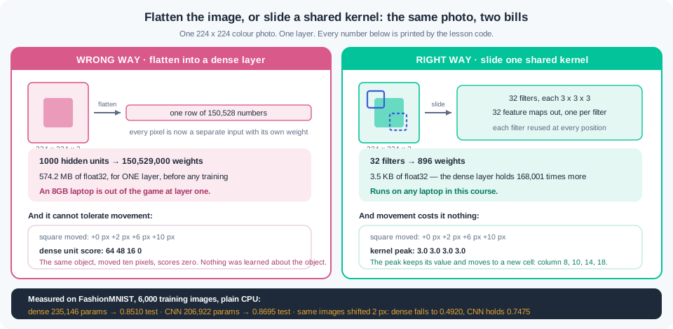
There is a wrong way and a right way to feed a picture to a network. The wrong way flattens it and gives every pixel its own private weight, which buys 150,529,000 parameters and no tolerance for movement. The right way slides one small set of weights across the whole image, so 896 parameters cover the same photo and the answer travels with the object. Rukmini's lead was holding the right way in his hand.
A convolution — a small window of weights slid across an image, multiplying and adding at every stop — is that sliding paper square. The window of weights is called a kernel, and a kernel is a pattern the layer looks for. Below you run a 3 by 3 edge kernel over a 6 by 6 patch by hand in NumPy. Where the window sits on the bright edge it reports 27, and where the patch is flat it reports 0. Run a horizontal-edge kernel on the same patch and every one of the 16 answers is 0, because that pattern is not there.
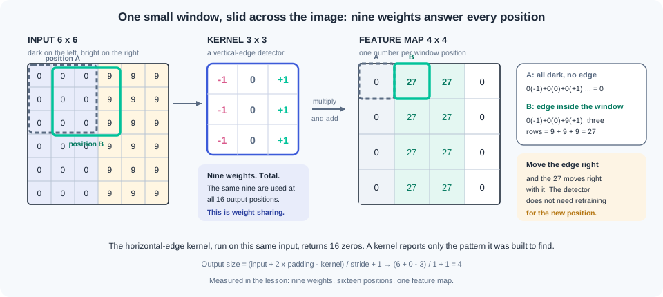
Two settings control how the window travels. Stride is the step size, or how many pixels the window jumps between stops, and a stride of 2 halves the output. Padding is a border of zeros added around the image so the window can also sit on the edges, and it lets a 3 by 3 kernel keep the picture the same size. One formula covers every case: output equals input plus twice the padding, minus the kernel size, divided by the stride, plus one. Learn it tonight, because it is the arithmetic that decides whether your model even builds.
Each kernel produces one feature map — a grid of scores showing where in the image that kernel found its pattern. A layer with 32 kernels makes 32 feature maps, and those become the 32 channels the next layer reads. PyTorch stores this as a shape with four parts: N, C, H, W, meaning batch, channels, height, and width. Your batch of 64 grey images enters as (64, 1, 28, 28) and leaves the first conv layer as (64, 16, 28, 28). Keep printing that shape after every layer, the way 0.4 and 2.1 taught you to print array shapes.
Depth changes what the kernels look for. Early layers see raw pixels, so they can only find simple things: edges, corners, and light-to-dark steps. Deeper layers read feature maps rather than pixels, so they combine those edges into textures, then into parts like a sleeve or a heel. In the trained network below, 9 of the first 16 filters respond most strongly to a vertical edge test, up from 5 before training. Nobody told the network to build edge detectors; the loss did.
Pooling — a step that shrinks a feature map by keeping one number from each small block — does two jobs. It cuts height and width by half, which cuts memory and compute for every later layer. It also buys tolerance: if the strongest response moves one pixel, the largest value in a 2 by 2 block is often unchanged. That is how a network stops caring exactly where the towel defect sits in the frame. Max pooling keeps the largest value in each block and is the common choice.
Then comes the measurement, because 2.3 taught you never to claim a win you have not printed. On the same 6,000 FashionMNIST images, a dense network with 235,146 parameters scores 0.8510 on the test set. A small CNN with fewer parameters, 206,922, scores 0.8695. The gap looks modest until you move every test image two pixels right: the dense model collapses to 0.4920 while the CNN holds 0.7475.
Data augmentation is the fifth overfitting tool that 2.4 named and left for today. You build new training images by changing old ones a little: shift them, crop them, flip them left to right. It carries one hard rule, and it is 1.7's rule wearing new clothes. Augment the training images only, never the validation or test images, because a test set exists to measure one fixed thing.
Break that rule and the numbers stop meaning anything. Below, the same trained model scored on the same test images gives 0.8575, then 0.8665, then 0.8410, because the random transform reshuffles the pictures on every call. Its honest score is 0.8730. Two pipelines, one for training and one for evaluation, is the whole fix.
Small image sets overfit fast, and 2.4's toolkit works here without change. Trained for 25 epochs with no augmentation, the CNN's training accuracy runs 7.9 points above its validation accuracy. Add train-only augmentation and that gap falls to 1.0 point, while robustness to a two-pixel shift climbs from 0.7285 to 0.8495. Early stopping with a rewind, dropout, and weight decay all still apply; augmentation is the tool images add.
CNNs are still the right answer in 2026 for a large slice of paid work. They run on edge devices with no GPU, and on medical or industrial images that cannot leave the building. They also do the clean-up stage in front of an OCR engine. When your task is broad natural photos with little data, a pretrained model beats anything you can train tonight, and module 2.6 shows you how to take one. Learn to build the small one first, so you can read, size, and debug the big one.
Work inside ai-lab with torch, torchvision, numpy and matplotlib. One-time setup: pip install torch==2.9.* torchvision==0.24.* — the 2.3 pin plus its matching torchvision — then the first FashionMNIST run downloads about 30 MB. Timings below come from a plain CPU laptop with four threads; an older Intel machine takes roughly three to five times longer, which is still minutes.
Step 1 — the parameter bill, and the position problem. Two arguments against dense layers on images, both as printed numbers:
import numpy as np

dense_params = lambda h, w, c, units: h * w * c * units + units
conv_params = lambda in_c, out_c, k: out_c * (in_c * k * k) + out_c

print(f"{'image':>12s} {'flattened':>10s} {'dense 1000 units':>18s} {'conv 3x3 x32':>13s}")
for h, w, c in [(28, 28, 1), (64, 64, 3), (224, 224, 3)]:
    print(f"{f'{h}x{w}x{c}':>12s} {h*w*c:10d} {dense_params(h,w,c,1000):18,d}"
          f" {conv_params(c,32,3):13,d}")

d, v = dense_params(224, 224, 3, 1000), conv_params(3, 32, 3)
print(f"\ndense layer weights as float32 : {d * 4 / 1024**2:8.1f} MB")
print(f"conv  layer weights as float32 : {v * 4 / 1024:8.1f} KB")
print(f"the dense layer holds {d / v:,.0f} times more numbers, for one layer")

def square_at(col):                       # an 8x8 bright square on a 28x28 canvas
    im = np.zeros((28, 28), dtype=np.float32)
    im[10:18, col:col + 8] = 1.0
    return im

base = square_at(10)
template = base.reshape(-1)               # a dense unit that learned this exact square
edge = np.array([[-1., 0., 1.], [-1., 0., 1.], [-1., 0., 1.]])

def conv2d(x, k):
    kh, kw = k.shape
    out = np.zeros((x.shape[0] - kh + 1, x.shape[1] - kw + 1))
    for i in range(out.shape[0]):
        for j in range(out.shape[1]):
            out[i, j] = float((x[i:i+kh, j:j+kw] * k).sum())
    return out

print(f"\n{'square moved':>14s} {'dense unit score':>17s} {'conv peak':>10s} {'peak column':>12s}")
for col in (10, 12, 16, 20):
    fmap = conv2d(square_at(col), edge)
    dense_score = float(template @ square_at(col).reshape(-1))
    print(f"{f'+{col-10} pixels':>14s} {dense_score:17.0f} {fmap.max():10.1f}"
          f" {int(np.argmax(fmap.max(axis=0))):12d}")
Output:
       image  flattened   dense 1000 units  conv 3x3 x32
     28x28x1        784            785,000           320
     64x64x3      12288         12,289,000           896
   224x224x3     150528        150,529,000           896

dense layer weights as float32 :    574.2 MB
conv  layer weights as float32 :      3.5 KB
the dense layer holds 168,001 times more numbers, for one layer

  square moved  dense unit score  conv peak  peak column
     +0 pixels                64        3.0            8
     +2 pixels                48        3.0           10
     +6 pixels                16        3.0           14
    +10 pixels                 0        3.0           18
Read the first table across the rows. The conv column barely moves — 320 for one grey channel, 896 for three colour channels — because a kernel's size depends on the channels and the window, never on the picture's height and width. The dense column explodes with the picture: 785,000 weights on a 28-pixel thumbnail, 150,529,000 on a normal photo, which is 574.2 MB for one layer. The second table is the argument that matters more. The dense unit's score decays 64, 48, 16, 0 as the identical square slides right, so at ten pixels it reports that nothing is there. The kernel's peak stays at exactly 3.0 and moves from column 8 to column 18, which is what "the answer travels with the object" means in numbers.
Step 2 — convolution by hand, before any framework. A 6 by 6 patch, a printed 3 by 3 kernel, and every step visible:
img = np.array([
    [0, 0, 0, 9, 9, 9],
    [0, 0, 0, 9, 9, 9],
    [0, 0, 0, 9, 9, 9],
    [0, 0, 0, 9, 9, 9],
    [0, 0, 0, 9, 9, 9],
    [0, 0, 0, 9, 9, 9]], dtype=float)

vertical = np.array([[-1, 0, 1],
                     [-1, 0, 1],
                     [-1, 0, 1]], dtype=float)
horizontal = vertical.T.copy()

def show(name, m, width=6):
    print(f"{name}  shape {m.shape}")
    for row in m:
        print("   " + " ".join(f"{v:{width}.0f}" for v in row))

show("INPUT (dark left, bright right)", img)
print()
show("KERNEL (vertical-edge detector)", vertical, 3)
print()

win = img[0:3, 1:4]                       # the window that fills output cell (0, 1)
show("window at output cell (0,1)", win, 3)
terms = " + ".join(f"{a:.0f}*{b:.0f}" for a, b in zip(win.reshape(-1), vertical.reshape(-1)))
print(f"   {terms} = {float((win*vertical).sum()):.0f}")
print()

fmap = conv2d(img, vertical)
show("FEATURE MAP (vertical kernel)", fmap)
print()
show("FEATURE MAP (same input, horizontal kernel)", conv2d(img, horizontal))
print(f"\nvertical kernel   : max {fmap.max():.0f}  min {fmap.min():.0f}")
print(f"horizontal kernel : max {conv2d(img, horizontal).max():.0f}")
print(f"parameters in this kernel: {vertical.size} weights, reused at all "
      f"{fmap.size} output positions")
Output:
INPUT (dark left, bright right)  shape (6, 6)
        0      0      0      9      9      9
        0      0      0      9      9      9
        0      0      0      9      9      9
        0      0      0      9      9      9
        0      0      0      9      9      9
        0      0      0      9      9      9

KERNEL (vertical-edge detector)  shape (3, 3)
    -1   0   1
    -1   0   1
    -1   0   1

window at output cell (0,1)  shape (3, 3)
     0   0   9
     0   0   9
     0   0   9
   0*-1 + 0*0 + 9*1 + 0*-1 + 0*0 + 9*1 + 0*-1 + 0*0 + 9*1 = 27

FEATURE MAP (vertical kernel)  shape (4, 4)
        0     27     27      0
        0     27     27      0
        0     27     27      0
        0     27     27      0

FEATURE MAP (same input, horizontal kernel)  shape (4, 4)
        0      0      0      0
        0      0      0      0
        0      0      0      0
        0      0      0      0

vertical kernel   : max 27  min 0
horizontal kernel : max 0
parameters in this kernel: 9 weights, reused at all 16 output positions
Say the middle line aloud, because it is the entire operation: nine multiplications, one sum, one output number. The window at cell (0, 1) covers columns 1, 2 and 3, so it holds three dark pixels and three bright ones; the negative side contributes 0 and the positive side contributes 27. Now read the feature map as a picture rather than a table. Columns 1 and 2 are lit at 27 because those two window positions straddle the edge, and columns 0 and 3 read 0 because those windows sit entirely inside one flat region. The second feature map is 16 zeros: the horizontal kernel found nothing here, which is the point — a kernel reports one pattern and stays silent about the rest. Nine weights covered all 16 positions, and that ratio is what stops the parameter count from exploding.
Step 3 — the output-size formula, checked against PyTorch. The arithmetic every vision interview asks you to do on paper:
import torch, torch.nn as nn

def out_size(n, k, s, p):
    return (n + 2 * p - k) // s + 1

print(f"{'in':>4s} {'k':>2s} {'s':>2s} {'p':>2s} {'formula':>8s} {'pytorch':>8s}")
for n, k, s, p in [(28, 3, 1, 0), (28, 3, 1, 1), (28, 5, 1, 2), (28, 3, 2, 1),
                   (28, 2, 2, 0), (32, 3, 1, 0), (32, 7, 2, 3), (224, 3, 1, 1)]:
    want = out_size(n, k, s, p)
    got = nn.Conv2d(1, 1, kernel_size=k, stride=s, padding=p)(
        torch.zeros(1, 1, n, n)).shape[-1]
    print(f"{n:4d} {k:2d} {s:2d} {p:2d} {want:8d} {got:8d}"
          f"  {'ok' if want == got else 'MISMATCH'}")

net = nn.Sequential(
    nn.Conv2d(1, 16, 3, padding=1), nn.ReLU(), nn.MaxPool2d(2),
    nn.Conv2d(16, 32, 3, padding=1), nn.ReLU(), nn.MaxPool2d(2),
    nn.Flatten(), nn.Linear(32 * 7 * 7, 128), nn.ReLU(), nn.Linear(128, 10))

x = torch.zeros(64, 1, 28, 28)
print(f"\n{'layer':<12s} {'output shape (N,C,H,W)':<24s} {'params':>9s}")
print(f"{'input':<12s} {str(tuple(x.shape)):<24s} {0:9d}")
for layer in net:
    x = layer(x)
    print(f"{layer.__class__.__name__:<12s} {str(tuple(x.shape)):<24s}"
          f" {sum(q.numel() for q in layer.parameters()):9,d}")
print(f"{'TOTAL':<12s} {'':<24s} {sum(q.numel() for q in net.parameters()):9,d}")
Output:
  in  k  s  p  formula  pytorch
  28  3  1  0       26       26  ok
  28  3  1  1       28       28  ok
  28  5  1  2       28       28  ok
  28  3  2  1       14       14  ok
  28  2  2  0       14       14  ok
  32  3  1  0       30       30  ok
  32  7  2  3       16       16  ok
 224  3  1  1      224      224  ok

layer        output shape (N,C,H,W)      params
input        (64, 1, 28, 28)                  0
Conv2d       (64, 16, 28, 28)               160
ReLU         (64, 16, 28, 28)                 0
MaxPool2d    (64, 16, 14, 14)                 0
Conv2d       (64, 32, 14, 14)             4,640
ReLU         (64, 32, 14, 14)                 0
MaxPool2d    (64, 32, 7, 7)                   0
Flatten      (64, 1568)                       0
Linear       (64, 128)                  200,832
ReLU         (64, 128)                        0
Linear       (64, 10)                     1,290
TOTAL                                    206,922
Eight formula rows, eight matches. Three of them are worth memorising as habits rather than sums: kernel 3 with padding 1 keeps the size, kernel 5 with padding 2 keeps the size, and a 2 by 2 max pool with stride 2 halves it. The shape trace below is the reflex this module drills. Follow the H and W columns down: 28, then 14 after the first pool, then 7 after the second, so the flatten is 32 channels times 7 times 7, which is 1568. That 1568 is the number you must compute before you can type nn.Linear, and getting it wrong is the most common error in this module (WR-130). Look at the params column too — the two conv layers cost 160 and 4,640 weights while the first dense layer costs 200,832, which is 97 percent of the model. Convolution is cheap; flattening is where the money goes.
Step 4 — a real CNN against a dense baseline, same data, honest clock. FashionMNIST is 28 by 28 grey clothing photos in ten classes. You take 6,000 training images, 1,000 for validation, 2,000 for test, and follow 2.3's canonical loop with 2.4's two-column watch:
import time, copy
from torch.utils.data import DataLoader, TensorDataset
from torchvision import datasets, transforms

torch.set_num_threads(4)
tt = transforms.ToTensor()
ftr = datasets.FashionMNIST("./data", train=True, download=True, transform=tt)
fte = datasets.FashionMNIST("./data", train=False, download=True, transform=tt)

g = torch.Generator().manual_seed(42)
perm = torch.randperm(len(ftr), generator=g)
tri, vai = perm[:6000].tolist(), perm[6000:7000].tolist()
tei = torch.randperm(len(fte), generator=g)[:2000].tolist()
stack = lambda ds, idx: (torch.stack([ds[i][0] for i in idx]),
                         torch.tensor([ds[i][1] for i in idx]))
Xtr, ytr = stack(ftr, tri); Xva, yva = stack(ftr, vai); Xte, yte = stack(fte, tei)
print("train", tuple(Xtr.shape), " val", tuple(Xva.shape), " test", tuple(Xte.shape))
print("pixel range", float(Xtr.min()), "to", float(Xtr.max()), " dtype", Xtr.dtype)

loss_fn = nn.CrossEntropyLoss()
dense_net = lambda: nn.Sequential(nn.Flatten(), nn.Linear(784, 256), nn.ReLU(),
                                  nn.Linear(256, 128), nn.ReLU(), nn.Linear(128, 10))
conv_net = lambda: nn.Sequential(
    nn.Conv2d(1, 16, 3, padding=1), nn.ReLU(), nn.MaxPool2d(2),
    nn.Conv2d(16, 32, 3, padding=1), nn.ReLU(), nn.MaxPool2d(2),
    nn.Flatten(), nn.Linear(32 * 7 * 7, 128), nn.ReLU(), nn.Linear(128, 10))

@torch.no_grad()
def score(net, X, y):
    net.eval()
    out = net(X)
    return loss_fn(out, y).item(), (out.argmax(1) == y).float().mean().item()

def train(name, build, epochs=12, lr=1e-3, bs=64):
    torch.manual_seed(7)                       # seed BEFORE the layers exist (2.4)
    net = build()
    opt = torch.optim.Adam(net.parameters(), lr=lr)
    dl = DataLoader(TensorDataset(Xtr, ytr), batch_size=bs, shuffle=True,
                    generator=torch.Generator().manual_seed(7))
    print(f"\n{name}  ({sum(p.numel() for p in net.parameters()):,} parameters)")
    print(f"{'epoch':>5s} {'train loss':>10s} {'val loss':>9s} {'val acc':>8s} {'sec':>6s}")
    best, state, t0 = float("inf"), None, time.perf_counter()
    for ep in range(1, epochs + 1):
        net.train()
        for xb, yb in dl:
            opt.zero_grad(); loss_fn(net(xb), yb).backward(); opt.step()
        trl, _ = score(net, Xtr, ytr)
        val, acc = score(net, Xva, yva)
        if val < best: best, state = val, copy.deepcopy(net.state_dict())
        print(f"{ep:5d} {trl:10.4f} {val:9.4f} {acc:8.3f} {time.perf_counter()-t0:6.1f}")
    net.load_state_dict(state)                 # 2.4's rewind to the best epoch
    print(f"  total {time.perf_counter()-t0:.1f} s   test accuracy {score(net, Xte, yte)[1]:.4f}")
    return net

dense = train("DENSE baseline  784-256-128-10", dense_net)
cnn = train("CNN  conv16-pool-conv32-pool-128-10", conv_net)

shifted = torch.roll(Xte, shifts=2, dims=3)    # every test image moved 2 px right
print(f"\n{'model':<8s} {'test acc':>9s} {'shifted +2px':>13s} {'drop':>7s}")
for label, net in (("dense", dense), ("cnn", cnn)):
    a, b = score(net, Xte, yte)[1], score(net, shifted, yte)[1]
    print(f"{label:<8s} {a:9.4f} {b:13.4f} {a-b:7.4f}")
Output, trimmed to the epochs that matter:
train (6000, 1, 28, 28)  val (1000, 1, 28, 28)  test (2000, 1, 28, 28)
pixel range 0.0 to 1.0  dtype torch.float32

DENSE baseline  784-256-128-10  (235,146 parameters)
epoch train loss  val loss  val acc    sec
    1     0.6239    0.6035    0.802    0.1
    6     0.3630    0.4369    0.837    0.3
   12     0.2597    0.3890    0.860    0.6
  total 0.6 s   test accuracy 0.8510

CNN  conv16-pool-conv32-pool-128-10  (206,922 parameters)
epoch train loss  val loss  val acc    sec
    1     0.6373    0.6072    0.785    0.8
    6     0.3872    0.4269    0.855    4.4
   12     0.2684    0.3533    0.874    8.9
  total 8.9 s   test accuracy 0.8695

model     test acc  shifted +2px    drop
dense       0.8510        0.4920  0.3590
cnn         0.8695        0.7475  0.1220
Four honest readings, in order. First the score: 0.8695 against 0.8510, so convolution wins by 1.85 accuracy points while holding fewer parameters, 206,922 against 235,146. Second the clock: the CNN took 8.9 seconds against 0.6, roughly fifteen times longer, because a conv layer does the same nine multiplications at every one of 784 positions. Third, and this is the result to carry into interviews, the shifted row: move every test image two pixels right and the dense model falls from 0.8510 to 0.4920, losing 35.9 points, while the CNN falls to 0.7475, losing 12.2. The dense model was memorising pixel addresses all along and the test set never revealed it, because the test images sat in the same places as the training images. Fourth, the shapes and pixel range printed at the top are the WR-126 audit in image form: (6000, 1, 28, 28) is N, C, H, W, and ToTensor already scaled pixels to 0.0 through 1.0, so no extra division by 255 belongs anywhere in this script.
Step 5 — augmentation, train-only, and the number it corrupts. Same CNN, same data, one transform pipeline added in exactly one place:
train_tf = transforms.Compose([transforms.RandomCrop(28, padding=2),
                               transforms.RandomHorizontalFlip(p=0.5)])
# there is deliberately no eval_tf: evaluation sees the raw images, always

def run(label, augment, epochs):
    torch.manual_seed(7)
    net = conv_net()
    opt = torch.optim.Adam(net.parameters(), lr=1e-3)
    dl = DataLoader(TensorDataset(Xtr, ytr), batch_size=64, shuffle=True,
                    generator=torch.Generator().manual_seed(7))
    best, state, t0 = float("inf"), None, time.perf_counter()
    for ep in range(1, epochs + 1):
        net.train()
        for xb, yb in dl:
            if augment: xb = train_tf(xb)          # TRAIN ONLY, inside the batch loop
            opt.zero_grad(); loss_fn(net(xb), yb).backward(); opt.step()
        val = score(net, Xva, yva)[0]
        if val < best: best, state = val, copy.deepcopy(net.state_dict())
    secs = time.perf_counter() - t0
    net.load_state_dict(state)
    tr_acc, va_acc = score(net, Xtr, ytr)[1], score(net, Xva, yva)[1]
    test_acc = score(net, Xte, yte)[1]
    shift_acc = score(net, torch.roll(Xte, 2, dims=3), yte)[1]
    print(f"{label:<26s} {epochs:3d} {secs:7.1f} {tr_acc-va_acc:+9.3f}"
          f" {test_acc:9.4f} {shift_acc:9.4f}")
    return net

print(f"{'run':<26s} {'ep':>3s} {'sec':>7s} {'tr-val gap':>9s} {'test':>9s} {'shifted':>9s}")
run("no augmentation", False, 12)
run("no augmentation, longer", False, 25)
aug = run("augmented (train only)", True, 25)

print("\nthe wrong way: the same transform applied to the test set")
for i in range(3):
    torch.manual_seed(100 + i)
    with torch.no_grad():
        aug.eval()
        acc = (aug(train_tf(Xte)).argmax(1) == yte).float().mean().item()
    print(f"  call {i+1}: reported 'test accuracy' {acc:.4f}")
print(f"  honest test accuracy, raw images: {score(aug, Xte, yte)[1]:.4f}")
Output:
run                         ep     sec tr-val gap      test   shifted
no augmentation             12     9.0     +0.034    0.8695    0.7475
no augmentation, longer     25    18.5     +0.079    0.8710    0.7285
augmented (train only)      25    18.8     +0.010    0.8730    0.8495

the wrong way: the same transform applied to the test set
  call 1: reported 'test accuracy' 0.8575
  call 2: reported 'test accuracy' 0.8665
  call 3: reported 'test accuracy' 0.8410
  honest test accuracy, raw images: 0.8730
Row two is the overfitting you were taught to spot in 2.4, now on images: doubling the epochs lifts the train-validation gap from 3.4 points to 7.9 and buys 0.0015 of test accuracy, which is noise. Row three is augmentation earning its place: same 25 epochs, same seed, gap down to 1.0 point, test accuracy up to 0.8730, and the two-pixel-shift score up from 0.7285 to 0.8495. That last column is the honest reason to augment on small sets — not a big jump on the easy test, but a model that survives a nudged camera, which is Rukmini's actual failure. Then read the wrong-way block. The same weights and the same 2,000 images report 0.8575, 0.8665 and 0.8410 on three consecutive calls, because a random crop and a random flip make a different test set every time. All three are below the honest 0.8730, and none of them is a measurement — WR-131 is the day a team shipped one of those numbers to a client.
Step 6 — what the first layer actually learned. No new training, only a look inside the kernels you already have:
torch.manual_seed(7)                                 # same seed the trained net started from
W0 = conv_net()[0].weight.detach().squeeze(1)        # a fresh, untrained layer
W = cnn[0].weight.detach().squeeze(1)                # the trained layer from Step 4
print("first conv weight tensor:", tuple(cnn[0].weight.shape),
      "= (out_channels, in_channels, kH, kW)")
print(f"before training: mean {W0.mean():+.4f}  std {W0.std():.4f}")
print(f"after  training: mean {W.mean():+.4f}  std {W.std():.4f}")

vert = torch.tensor([[-1., 0., 1.]] * 3)
horz = vert.T.contiguous()
blob = torch.ones(3, 3)

def tags(Wx):
    names = []
    for i in range(Wx.shape[0]):
        s = {"vertical": abs(float((Wx[i]*vert).sum())),
             "horizontal": abs(float((Wx[i]*horz).sum())),
             "brightness": abs(float((Wx[i]*blob).sum()))}
        names.append(max(s, key=s.get))
    return {t: names.count(t) for t in ("vertical", "horizontal", "brightness")}

print("\nstrongest response of each of the 16 filters:")
print("  before training:", tags(W0))
print("  after  training:", tags(W))
for i in (14, 1):
    print(f"\nlearned filter {i}:")
    for row in W[i]:
        print("   " + "  ".join(f"{x:+.3f}" for x in row))

x = torch.zeros(1, 1, 28, 28); x[0, 0, 10:18, 10:18] = 1.0
with torch.no_grad():
    a1 = cnn[0](x)
    a2 = cnn[3](cnn[2](cnn[1](a1)))
print(f"\none bright square in, feature maps out:")
print(f"  after conv1: {tuple(a1.shape)}  filters that fired: "
      f"{int((a1.amax(dim=(2,3)) > 0.1).sum())} of 16")
print(f"  after conv2: {tuple(a2.shape)}  filters that fired: "
      f"{int((a2.amax(dim=(2,3)) > 0.1).sum())} of 32")
Output:
first conv weight tensor: (16, 1, 3, 3) = (out_channels, in_channels, kH, kW)
before training: mean -0.0032  std 0.1784
after  training: mean +0.0204  std 0.2480

strongest response of each of the 16 filters:
  before training: {'vertical': 5, 'horizontal': 4, 'brightness': 7}
  after  training: {'vertical': 9, 'horizontal': 1, 'brightness': 6}

learned filter 14:
   -0.449  -0.235  +0.236
   +0.019  -0.201  +0.053
   -0.384  +0.244  +0.429

learned filter 1:
   +0.369  +0.387  +0.174
   -0.034  -0.099  -0.007
   -0.050  +0.165  -0.359

one bright square in, feature maps out:
  after conv1: (1, 16, 28, 28)  filters that fired: 14 of 16
  after conv2: (1, 32, 14, 14)  filters that fired: 31 of 32
The weight tensor's shape is the first thing to read: (16, 1, 3, 3) means 16 filters, each seeing 1 input channel through a 3 by 3 window, which is 144 weights plus 16 biases and matches Step 3's 160. Training pushed the spread of those weights from 0.1784 to 0.2480, so the filters grew opinions instead of staying near their random start. The tag counts show what those opinions are: 5 filters leaned vertical before training and 9 after, purely from the loss. Filter 14 is the clean case — read its columns, negative on the left and positive on the right, which is the hand-built edge kernel from Step 2 rediscovered by gradient descent. Filter 1 is its rotation, positive across the top row and negative across the bottom, so it answers to horizontal edges. Do not over-read this probe: three test patterns cannot describe a filter fully, and the honest claim is that early layers land on simple local patterns while the later layers, reading 32 channels at once, build the textures and parts that no 3 by 3 grid of numbers can show you.
Work inside ai-lab with torch, torchvision and numpy. Everything is seeded, so where a loss or an accuracy is given your output should land within about 1% of it — seeded torch runs vary slightly across builds — while shapes and counts should match exactly; wall-clock seconds will differ with your machine and that is expected. Keep Step 4's data-loading block in a file you import, because exercises 2 to 4 all reuse Xtr, ytr, Xva, yva, Xte, yte.
If your numbers are close but not identical, triage in a fixed order before touching your code. Everything off by a little — every value drifting in the last decimal or two — points at a library version: run pip show torch, compare it with the pinned install line, and match the pin, because the printed numbers were produced on that version. One number wildly off while the rest agree points at stale state: restart from a fresh kernel or a fresh python and run the file top to bottom, since seeded draws only reproduce when they happen in the same order from a clean start. Only when both checks pass and the numbers still disagree should you suspect your own logic — diff your script line by line against the printed code.
Convolution by hand, then proved against PyTorch. Create conv_by_hand.py. Part one: write conv2d(x, k) yourself with two loops, no framework calls, and no np.convolve. Part two: build the 6 by 6 patch from Step 2 and run three kernels over it — the vertical edge, the horizontal edge, and a 3 by 3 blur whose nine weights are each one ninth. Print the input, each kernel, and each feature map, and write one comment line per feature map saying in words what it found. Part three: build a second 6 by 6 patch with a horizontal edge instead (top three rows 0, bottom three rows 9) and run both edge kernels on it, showing that the roles swap. Part four: prove your loops are correct by calling torch.nn.functional.conv2d on the same input and kernel, and print the largest absolute difference between your output and the framework's. Watch the trap here: the framework's conv2d does cross-correlation, the same operation you wrote, but it needs a 4-D input shaped (N, C, H, W) and a 4-D weight shaped (out, in, kH, kW), so img[None, None] and kernel[None, None] are the reshapes you need. Check: the vertical kernel on the vertical-edge patch prints a 4 by 4 map whose middle two columns are 27 and whose outer columns are 0; the horizontal kernel on that same patch prints 16 zeros; the roles swap exactly on the second patch, with 27s in the middle two rows; the blur kernel returns 0 on the dark side, 9 on the bright side, and 3 and 6 in the two straddling columns; the largest gap against torch.nn.functional.conv2d prints below 1e-6; and your comment lines describe the maps in words, not in restated numbers.
The shape drill — predict every shape before you run anything. Create shape_drill.py. Part one, on paper first and in comments in the file: for each of the three stacks below, write the output shape after every single layer, in N, C, H, W form, using only the formula from Step 3. Do not run code until all three are written down.
STACK A  input (32, 1, 28, 28)
  Conv2d(1, 8, kernel_size=5, padding=0) -> ReLU -> MaxPool2d(2)
  Conv2d(8, 16, kernel_size=3, padding=1) -> ReLU -> MaxPool2d(2)
  Flatten -> Linear(?, 64) -> Linear(64, 10)

STACK B  input (16, 3, 64, 64)
  Conv2d(3, 32, kernel_size=7, stride=2, padding=3) -> ReLU
  MaxPool2d(2) -> Conv2d(32, 64, kernel_size=3, stride=2, padding=1) -> ReLU
  Flatten -> Linear(?, 128)

STACK C  input (8, 1, 28, 28)
  Conv2d(1, 32, kernel_size=3, padding=1) -> ReLU -> MaxPool2d(2)
  Conv2d(32, 64, kernel_size=3, padding=1) -> ReLU -> MaxPool2d(2)
  Conv2d(64, 64, kernel_size=3, padding=1) -> ReLU -> MaxPool2d(2)
  Flatten -> Linear(?, 10)
Part two: build all three in PyTorch, replacing each ? with the number you predicted, push a zero tensor of the stated shape through, and print the real shape after every layer beside your prediction with a pass or fail mark. Part three: break stack A on purpose by changing the first padding=0 to padding=2 without touching the Linear, run it, and paste the exact error message into a comment; then state in one sentence which of the two numbers in that message is your flatten size and which is the layer's expectation. Part four: write a helper flatten_size(h, w, layers) that takes a starting height and width and a list of layer specs and returns the flatten count, then use it to confirm all three stacks. Check: stack A traces 28 to 24 to 12 to 12 to 6, with a flatten of 16 times 6 times 6 equal to 576; stack B traces 64 to 32 to 16 to 8, with a flatten of 64 times 8 times 8 equal to 4096; stack C traces 28 to 14 to 7 to 3 — note the floor at the last pool — with a flatten of 64 times 3 times 3 equal to 576; every printed shape matches your written prediction; the broken run raises RuntimeError: mat1 and mat2 shapes cannot be multiplied (32x784 and 576x64) and your comment names 784 as the new flatten size and 576 as the layer's stale expectation; and flatten_size reproduces all three counts with no hard-coded numbers.
Build and beat. Create beat_the_baseline.py. Rebuild Step 4's data exactly: FashionMNIST, generator seed 42, 6,000 training images, 1,000 validation, 2,000 test, ToTensor only. Part one: train the dense baseline 784-256-128-10 with Adam at 0.001, batch 64, 12 epochs, printing the two-column epoch table from 2.4 and keeping the best-validation weights with a rewind. Record its test accuracy and its wall-clock seconds. Part two: design your own CNN and beat that number on the same 2,000 test images. You may change the number of conv layers, the filter counts, the kernel sizes, the padding, the pooling, and the size of the dense head. You may not use more than 400,000 parameters, may not train for more than 25 epochs, and may not touch the test set until your architecture is frozen — the validation curve makes every decision, which is 1.7's law and 2.4's discipline together. Part three: keep a results table with one row per attempt holding architecture, parameter count, seconds, best validation loss, and test accuracy, changing one thing per row as WR-128 requires. Part four: evaluate your winner and the dense baseline on torch.roll(Xte, 2, dims=3) and report both drops. Close with three comment sentences: which change earned the most, what it cost in seconds, and what the shifted column says that the plain test column hides. Check: your dense baseline reproduces 0.8510 test accuracy and finishes in under two seconds; your CNN's test accuracy is above 0.8695, the reference model's score, with a parameter count you print and keep under 400,000 — a third conv block of 64 filters reaches 0.8805 on only 98,442 parameters in about 18 seconds on a plain CPU, while widening the existing blocks to 32 and 64 filters reaches 0.8880 but costs 421,642 parameters and breaks the cap until you shrink the dense head; your results table has at least four rows and each row differs from the one above it in exactly one setting; the shifted evaluation shows the dense model losing more than 30 accuracy points while your CNN loses under 20; and your comments name the validation set, never the test set, as what chose your architecture.
Augment properly, then hunt the cheat. Create augment_and_audit.py and reuse your winner from exercise 3. Part one: add transforms.Compose([transforms.RandomCrop(28, padding=2), transforms.RandomHorizontalFlip(p=0.5)]) to the training batches only, train for 25 epochs, and print one table with four columns for both the plain and augmented runs: train-minus-validation accuracy gap, test accuracy, shifted-by-two-pixels accuracy, and seconds. Part two: reproduce the failure on purpose. Apply the same transform inside your evaluation function, score the identical model on the identical test set three times with three different seeds, and print all three numbers next to the honest one. Write two comment sentences naming what that number now measures and why a client demo built on it is a lie. Part three: the leakage hunt. Copy your training images, paint a faint 3 by 3 patch of value 0.55 into the top-left corner of every image of class 6 only, do the same to the validation and test copies, and retrain. Then score that model on the clean, unpainted test set, and finally paint the same corner patch onto class 0 images instead and score those. Part four: print the ten worst-scoring classes with their accuracies and the five most common true-to-predicted confusions for your honest model, then write two sentences on which pairs a human would also confuse. Check: the augmented run's train-validation gap is at least three points smaller than the plain run's, and its shifted accuracy is at least eight points higher (reference numbers: gap +0.079 falling to +0.010, shifted 0.7285 rising to 0.8495); the three augmented-evaluation scores differ from each other and all sit below the honest score (reference: 0.8575, 0.8665, 0.8410 against 0.8730); the painted model scores near 1.0000 on painted class 6 and collapses to near 0.0050 on clean class 6, and painting the mark onto class 0 makes the model call almost every one of those images class 6 (reference: 174 of 174); and your confusion list has Shirt against T-shirt and Pullover against Coat near the top, with a comment agreeing that those pairs are genuinely hard rather than a bug.
Three vision failures cover most of this module's pain. Each has a War Room entry with the full diagnosis path:
- WR-130 — the flatten that did not fit. A conv stack's output size was computed by guesswork, so the first dense layer expected 1568 inputs and received 800: the loud version is
mat1 and mat2 shapes cannot be multiplied, and the quiet version is anAdaptiveAvgPool2ddropped in to make the numbers agree, which cost 1.9 accuracy points and hid the real padding bug; the fix is the output-size formula applied layer by layer and a shape print after every layer before training starts. - WR-131 — the augmented test set. Training transforms were attached to the evaluation loader as well, so the reported accuracy changed on every run and sat below the true score: the number measured randomly damaged images, not the model; the fix is two separate transform pipelines, one for training and one for evaluation, and an assertion that the evaluation pipeline holds nothing random.
- WR-132 — the model that learned the background. One class was shot under different lighting with a corner watermark, so the network learned the mark instead of the object: it read 1.0000 on that class in the lab and 0.0050 once the mark was gone; the fix is to inspect misclassified and suspiciously perfect images, control the capture conditions, and treat this as 1.7's leakage in image form.
A dense layer on a 224-pixel colour photo needs 150,529,000 weights and still cannot recognise the same object two pixels to the left. A convolution slides one small kernel across the whole image, so 896 weights cover that photo and the response travels with the object. Stride, padding, and the output-size formula decide every intermediate shape, and pooling halves height and width while adding tolerance to small shifts. On 6,000 FashionMNIST images a small CNN scored 0.8695 against a dense baseline's 0.8510, and on the same images shifted two pixels it held 0.7475 while the dense model fell to 0.4920. Augment the training images only, watch both curves as 2.4 taught, and check that your model learned the object rather than the corner of the frame.
- Document pipelines at Indian banks and fintechs clean up Aadhaar and PAN scans before OCR runs. Small convolutional models find the card edges, straighten the crop, and drop blurred frames, and they run on the branch machine because the images cannot leave it.
- Crop-disease apps for farmers classify a leaf photo taken on a low-cost phone, often with patchy network. A CNN of a few hundred thousand parameters fits on the handset, and augmentation is what makes it survive the odd angles and light of a real field.
- Defect cameras on factory lines in textile and auto-parts units flag faults at conveyor speed. There is no GPU on the shop floor and no time to call a cloud model, so a small CNN with pooling is the standard answer.
Answer these before opening the gate assessment. Each question names its type.
type=output-prediction— A stack takes input(16, 3, 64, 64)and appliesConv2d(3, 32, kernel_size=7, stride=2, padding=3), thenMaxPool2d(2), thenConv2d(32, 64, kernel_size=3, stride=2, padding=1). Predict the shape after each of the three layers in N, C, H, W form, and give the flatten size that the nextnn.Linearmust expect.type=debug— Training crashes withRuntimeError: mat1 and mat2 shapes cannot be multiplied (64x800 and 1568x128). Name which number came from the conv stack and which from the dense layer, state the most likely single edit that caused it, and give the two-line check you would add before any future training run.type=interpretation— Two models score 0.8510 and 0.8695 on the same test set, but on that test set shifted two pixels right they score 0.4920 and 0.7475. State what the second pair reveals that the first pair hides, and say which model you would put behind a factory camera and why.type=scenario-judgement— A teammate reports a test accuracy that moves between 0.84 and 0.87 on repeated runs of the same saved model on the same images. Judge what is happening, name the line of code you would ask to see first, and state what the reported number was actually measuring.type=trade-off— A small CNN trained from scratch versus a pretrained model fine-tuned for the task, for a defect camera on a shop floor with 900 labelled photos and no GPU. Give one concrete advantage and one concrete cost of each, and say which you would start with and what would change your mind.
Explain to a friend who has trained a dense network on a table of numbers and now wants to feed it photos: why does flattening the photo fail, and what does a convolution do instead? Use at most 4 sentences, name one parameter count and one accuracy number from this module, and use no maths word beyond "multiply" and "add". If they ask "so is a CNN always better", your answer names the shifted-image result and the 2.6 case for a pretrained model.