Making training actually work
Chaitra builds an arrears model at an electricity board office in Shivamogga. Her network trained for two hundred epochs, and the training loss ended near zero. On Monday it flagged the wrong homes, and her lead opened the run log. One curve sat there, alone. "You watched the model learn the answer sheet," he said. "Nobody watched it forget the point." He drew a second line beside the first, rising where the first fell. Tonight Chaitra learns to read both.
- "Your model overfits — what do you do?" is a standard fresher deep-learning round at Indian AI teams, and tonight you earn a measured answer with five named tools.
- Most "the model is bad" evenings are training-setup bugs, not limits of the model. Reading two curves saves you the week that a bigger network would waste.
- The whole module is CPU-only on an 8GB laptop. Every run here finishes in about two seconds, and every number below came from that machine.
Module 2.3 ended with a working loop and an honest score. The network reached 0.79 on the churn table while a plain logistic pipeline reached 0.83. Nothing in that loop was broken. What was missing is everything this module adds: the dials that turn "it trains" into "it trains well". Most of them cost one line each.
Start by splitting the data three ways instead of two. A validation set — a slice of the training rows held back to watch the model while it learns — is the second curve on your chart. The test set stays sealed until the end, as module 1.7 taught. Today 500 customer rows become 281 for training, 94 for validation, and 125 for the final test. Every choice you make from here is judged on the validation curve, never on the test set.
One curve tells you almost nothing. Two curves, read together, name the illness.
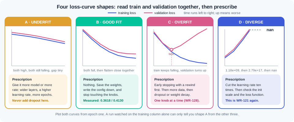
Four shapes cover nearly every run you will meet. Underfit: both curves sit high and fall slowly, so the model is too small or the rate too low. Good fit: both fall, then flatten close together. Overfitting — the state where training loss keeps falling while validation loss climbs — shows as two curves pulling apart. Diverge: the loss explodes to huge numbers and then to nan, which is 2.2's WR-121 wearing a new coat.
There is a wrong way and a right way to spend an evening of training. The wrong way runs 200 epochs blind, watches only the training loss, and ships whatever comes out. Chaitra's Monday came from that habit: today's blind run ends with a training loss of 0.0007 and a validation loss of 2.3038. The right way plots both curves from epoch one and stops when the validation curve turns. In the measured run below, stopping early scored 0.824 on the test set while the full 400 epochs scored 0.712.
The overfitting toolkit holds five tools, and you will measure each one on its own. More data comes first, because it is the only fix that costs the model nothing. Early stopping — the rule that halts training once the validation score stops improving, then rewinds to the best epoch — is the cheapest of the rest. Dropout — a layer that silences a random share of neurons during each training step — forces the network to spread its bets instead of leaning on a few paths. Weight decay — a gentle pull on every weight towards zero, added into the loss — keeps the network from trusting any single input too much.
The fifth tool is data augmentation: build new training rows by changing old ones a little. It earns a full workshop on images in 2.5, so today it is named, not built.
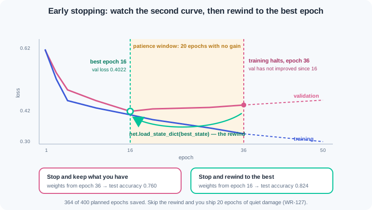
Early stopping needs two settings and one habit. Patience is how many epochs of no gain you tolerate before you halt, and 20 is a fair start. The habit is restoring the best weights, because the epochs after the best one made the model worse. Today's run stops at epoch 36 and rewinds to epoch 16. Skip the rewind and the same run scores 0.760 instead of 0.824.
Batch size moves three things at once, and you will measure all three. Memory grows in a straight line with it: a batch of 8 held 2.2 KB of activations here, a batch of 281 held 77.9 KB. Small batches make the curve jump about, because each step sees a small and sometimes unlucky sample. Large batches run faster per epoch on a laptop, since there are fewer Python steps to pay for. On 8GB with images in 2.5, memory will pick this dial for you.
A learning rate schedule — a rule that lowers the rate as training goes on — lets you start fast and finish carefully. Step schedules cut the rate by ten at chosen epochs, and cosine schedules glide it down to zero. Warmup does the opposite at the start: it raises the rate over the first few hundred steps, and very large models need it. On today's table a schedule bought steadiness rather than a jump in score. The late-run wobble fell from 0.0028 to 0.0000 while the test score moved from 0.744 to 0.768.
Optimizers deserve one honest line. Adam between 0.001 and 0.01 is the default that works, and 2.3 already measured it beating plain SGD on the same net. SGD with momentum still wins on large vision models trained for long runs, and it pairs well with a schedule. Reach for Adam first, and switch when a paper or a leaderboard gives you a reason.
Weight init looked like a detail in 2.1, and WR-120 was the bill. Stack six layers with weights drawn from normal(0, 1.0), and the signal grows at every layer: below you measure a spread of 1.39, then 8.90, then 54.9, up to 8521 by layer six. PyTorch's default scales each layer's weights by its width, so the same stack stays inside a healthy band. That default is the reason your networks have behaved so far. Do not overwrite it with a hand-picked number unless you can say why.
Normalisation layers do that job during training, not only at the start. BatchNorm rescales each feature using the current batch's mean and spread, while LayerNorm does it across each row instead, and Phase 3's transformers use LayerNorm everywhere. Add BatchNorm and the same broken stack holds a steady 0.58 at every layer. These layers carry a trap: they behave one way in training mode and another in eval mode. Score a net with dropout and BatchNorm in train mode and the same data gives 0.4477, then 0.5032, then 0.5216 — WR-125, now with teeth.
Two habits carry all of this. Change one knob at a time and write the row down, because five changes at once teach you nothing (WR-128). Seed the run and save the config, or the good run never comes back (WR-129). You will keep a recipe checklist from tonight and open it before every run, the way 2.3's five-step loop is now muscle memory.
Work inside ai-lab with torch, numpy, pandas and scikit-learn. This is one continuous session: Step 1 builds the world and every later step reuses its names. Each step finishes in about two seconds on a plain CPU.
Step 1 — the three-way split, and the four shapes made on purpose. Take 2.3's Ludhiana churn world, carve a validation set out of the training rows, then produce underfit, good fit, overfit and divergence on the same data:
import numpy as np, pandas as pd, torch, torch.nn as nn
from sklearn.model_selection import train_test_split
from sklearn.preprocessing import StandardScaler

rng = np.random.default_rng(42)                      # 2.3's Ludhiana world, unchanged
n = 500
snapshot = pd.Timestamp("2026-06-30")
customers = pd.DataFrame({
    "city": rng.choice(["Ludhiana", "Jalandhar", "Amritsar",
                        "Patiala", "Bathinda"], size=n),
    "monthly_income": rng.integers(18000, 120000, size=n),
    "orders_last_90d": rng.poisson(6, size=n),
    "avg_order_value": rng.integers(120, 900, size=n)})
customers["last_order_date"] = snapshot - pd.to_timedelta(
    rng.integers(1, 120, size=n), unit="D")
spend_share = (customers["avg_order_value"] * customers["orders_last_90d"]
               / 3) / customers["monthly_income"]
days_since = (snapshot - customers["last_order_date"]).dt.days
salary_week = (customers["last_order_date"].dt.day <= 7).astype(int)
risk = (-3.0 + 0.05 * days_since - 25 * spend_share
        - 1.3 * salary_week - 0.15 * customers["orders_last_90d"])
customers["churned"] = (rng.random(n) < 1 / (1 + np.exp(-risk))).astype(int)
customers["days_since_last_order"] = days_since
customers["spend_share"] = spend_share
customers["salary_week_order"] = salary_week

feats = ["monthly_income", "orders_last_90d", "avg_order_value",
         "days_since_last_order", "spend_share", "salary_week_order"]
X_fit, X_test, y_fit, y_test = train_test_split(          # 2.3's test split
    customers[feats], customers["churned"],
    test_size=0.25, random_state=42, stratify=customers["churned"])
X_train, X_val, y_train, y_val = train_test_split(        # NEW: carve a val set
    X_fit, y_fit, test_size=0.25, random_state=42, stratify=y_fit)

scaler = StandardScaler().fit(X_train)                    # train rows only, 1.7's law
T = lambda d: torch.tensor(scaler.transform(d), dtype=torch.float32)
L = lambda s: torch.tensor(s.values, dtype=torch.float32).reshape(-1, 1)
Xtr, ytr = T(X_train), L(y_train)
Xva, yva = T(X_val), L(y_val)
Xte, yte = T(X_test), L(y_test)
print("train", tuple(Xtr.shape), " val", tuple(Xva.shape), " test", tuple(Xte.shape))
print("churn rate  train %.3f  val %.3f  test %.3f" % (ytr.mean(), yva.mean(), yte.mean()))

loss_fn = nn.BCEWithLogitsLoss()

def shape(name, build_net, lr, marks, opt_name="Adam", epochs=400):
    torch.manual_seed(7)                 # seed BEFORE the layers exist
    net = build_net()
    opt = (torch.optim.Adam(net.parameters(), lr=lr) if opt_name == "Adam"
           else torch.optim.SGD(net.parameters(), lr=lr))
    print(f"\n{name}\nepoch   train     val")
    for ep in range(1, epochs + 1):
        net.train()
        opt.zero_grad(); loss_fn(net(Xtr), ytr).backward(); opt.step()
        if ep in marks:
            net.eval()
            with torch.no_grad():
                tr = loss_fn(net(Xtr), ytr).item()
                va = loss_fn(net(Xva), yva).item()
            f = lambda v: f"{v:.4f}" if abs(v) < 1e4 else f"{v:.2e}"
            print(f"{ep:5d}  {f(tr):>10s}  {f(va):>10s}")

M = (1, 20, 60, 100, 200, 400)
small = lambda: nn.Sequential(nn.Linear(6, 2), nn.ReLU(), nn.Linear(2, 1))
right = lambda: nn.Sequential(nn.Linear(6, 16), nn.ReLU(), nn.Linear(16, 1))
big   = lambda: nn.Sequential(nn.Linear(6, 64), nn.ReLU(),
                              nn.Linear(64, 64), nn.ReLU(), nn.Linear(64, 1))

shape("A  UNDERFIT   6-2-1, Adam 0.0005",    small, 0.0005, M)
shape("B  GOOD FIT   6-16-1, Adam 0.003",    right, 0.003,  M)
shape("C  OVERFIT    6-64-64-1, Adam 0.01",  big,   0.01,   M)
shape("D  DIVERGE    6-64-64-1, SGD 200",    big,   200.0, (1, 2, 3, 5, 10, 20), "SGD", 20)
Output, header first: train (281, 6) val (94, 6) test (125, 6) and churn rate train 0.313 val 0.309 test 0.312. The split is stratified, so all three slices carry the same churn rate — a check worth printing every time, because an unbalanced validation slice makes every later number a lie. Then the four tables:
Shape A, underfit, reads 0.7575 / 0.7632 at epoch 1 and 0.6378 / 0.6633 at epoch 400. Both numbers are high, both still falling, and the gap between them is tiny. The prescription is more model or more rate, never more stopping.
Shape B, the good fit, reads 0.6804 / 0.6936, then 0.4101 / 0.4445 at epoch 100, then 0.3618 / 0.4130 at epoch 400. Both curves fall and flatten, and they stay about 0.05 apart. This is what a healthy run looks like, and it is the target for every table you build later.
Shape C is the illness. It reads 0.3735 / 0.4096 at epoch 20 — its best moment — then 0.2111 / 0.4863, then 0.0596 / 0.9111, and finally 0.0007 / 2.3038. Read the two columns as one story: training loss falls a thousandfold while validation loss rises sixfold. The model is memorising 281 rows. Anyone watching one column would call this the best run of the evening.
Shape D is divergence, and it needs only 20 epochs to end. It reads 610.2867 / 583.5426, then 1.18e+09, then 2.79e+17, then 2.29e+34, then nan from epoch 10 onward. The rate of 200 makes every step overshoot, values overflow float32, and one nan poisons the rest of the run — WR-121's opening scene, reproduced in three seconds. Note the ordering trap this step also fixes: torch.manual_seed(7) runs before build_net() is called, because layers draw their random weights the moment they are constructed. Seed after building and every rerun gives different numbers.
Step 2 — early stopping, with patience and a rewind. Same overfitting net, same rate, one measurement loop added:
import copy

def test_acc(net):
    net.eval()
    with torch.no_grad():
        return ((torch.sigmoid(net(Xte)) > 0.5).float() == yte).float().mean().item()

torch.manual_seed(7)
net = big()
opt = torch.optim.Adam(net.parameters(), lr=0.01)
best, best_epoch, best_state, wait, patience = float("inf"), 0, None, 0, 20

for epoch in range(1, 401):
    net.train()
    opt.zero_grad(); loss_fn(net(Xtr), ytr).backward(); opt.step()
    net.eval()
    with torch.no_grad():
        tr = loss_fn(net(Xtr), ytr).item()
        va = loss_fn(net(Xva), yva).item()
    if va < best - 1e-4:                       # a real improvement
        best, best_epoch, wait = va, epoch, 0
        best_state = copy.deepcopy(net.state_dict())
    else:
        wait += 1                              # one more epoch with no gain
    if epoch <= 3 or epoch % 10 == 0 or wait >= patience:
        print(f"epoch {epoch:3d}  train {tr:.4f}  val {va:.4f}"
              f"  best {best:.4f} @{best_epoch}  wait {wait}")
    if wait >= patience:
        print(f"early stop: no val gain for {patience} epochs")
        break

print(f"stopped at epoch {epoch} of 400  -> {400 - epoch} epochs saved")
print(f"weights as stopped : test accuracy {test_acc(net):.3f}")
net.load_state_dict(best_state)                # rewind to the best epoch
print(f"restored epoch {best_epoch:2d}  : test accuracy {test_acc(net):.3f}  val loss {best:.4f}")
Output: epoch 1 train 0.6105 val 0.6088 best 0.6088 @1 wait 0, on through epoch 20 train 0.3735 val 0.4096 best 0.4022 @16 wait 4 and epoch 30 ... best 0.4022 @16 wait 14, then epoch 36 train 0.3267 val 0.4241 best 0.4022 @16 wait 20, early stop: no val gain for 20 epochs, stopped at epoch 36 of 400 -> 364 epochs saved, weights as stopped : test accuracy 0.760, and restored epoch 16 : test accuracy 0.824 val loss 0.4022. Three numbers carry the whole lesson. First, 364 epochs saved — on a laptop that is seconds, on a fine-tune in Phase 3 it is hours of rented GPU. Second, the rewind is not optional: the weights at epoch 36 score 0.760, the weights at epoch 16 score 0.824, and the difference is 20 epochs of quiet damage. Third, compare 0.824 against 2.3's 0.79 and against 1.6's logistic 0.83 — one line of training discipline closed most of that gap, with no change to the network at all. The wait column is the whole mechanism: it counts epochs since the last real gain, and best - 1e-4 stops float noise from resetting the counter.
Step 3 — the toolkit, one knob at a time. Same net, same seed, one change per row, and an honest table at the end:
def make(dropout=0.0):
    layers = [nn.Linear(6, 64), nn.ReLU()]
    if dropout: layers.append(nn.Dropout(dropout))
    layers += [nn.Linear(64, 64), nn.ReLU()]
    if dropout: layers.append(nn.Dropout(dropout))
    return nn.Sequential(*layers + [nn.Linear(64, 1)])

def study(label, dropout=0.0, decay=0.0, early=False, rows=281,
          epochs=400, patience=20):
    torch.manual_seed(7)                       # seed, then build
    net = make(dropout)
    opt = torch.optim.Adam(net.parameters(), lr=0.01, weight_decay=decay)
    Xs, ys = Xtr[:rows], ytr[:rows]
    best, best_epoch, best_state, wait = float("inf"), 0, None, 0
    ran = epochs
    for epoch in range(1, epochs + 1):
        net.train()
        opt.zero_grad(); loss_fn(net(Xs), ys).backward(); opt.step()
        net.eval()
        with torch.no_grad(): va = loss_fn(net(Xva), yva).item()
        if va < best - 1e-4:
            best, best_epoch, wait = va, epoch, 0
            best_state = copy.deepcopy(net.state_dict())
        else:
            wait += 1
        if early and wait >= patience:
            ran = epoch; break
    if early: net.load_state_dict(best_state)
    net.eval()
    with torch.no_grad():
        tr = loss_fn(net(Xs), ys).item()
        va = loss_fn(net(Xva), yva).item()
        pred = (torch.sigmoid(net(Xte)) > 0.5).float()
    acc = (pred == yte).float().mean().item()
    caught = int(((pred == 1) & (yte == 1)).sum().item())
    print(f"{label:26s} {ran:4d}  {tr:8.4f}  {va:8.4f}  {best:8.4f}@{best_epoch:<4d}"
          f" {acc:.3f}  {caught:2d}/39")

print(f"{'knob (one at a time)':26s} {'ep':>4s}  {'train':>8s}  {'val':>8s}"
      f"  {'best val':>8s}      {'test':5s} caught")
study("baseline, nothing on")
study("only 100 training rows", rows=100)
study("only 200 training rows", rows=200)
study("+ dropout 0.2",     dropout=0.2)
study("+ dropout 0.5",     dropout=0.5)
study("+ weight decay 1e-3", decay=1e-3)
study("+ weight decay 1e-2", decay=1e-2)
study("+ weight decay 1e-1", decay=1e-1)
study("+ early stopping",   early=True)
study("dropout+decay+early", dropout=0.5, decay=1e-2, early=True)
Output, the table this module exists for:
knob (one at a time)         ep     train       val  best val      test  caught
baseline, nothing on        400    0.0007    2.3038    0.4022@16   0.712  19/39
only 100 training rows      400    0.0001    3.4035    0.5024@5    0.728  24/39
only 200 training rows      400    0.0026    2.0909    0.4455@19   0.712  20/39
+ dropout 0.2               400    0.0544    1.0735    0.4017@16   0.688  19/39
+ dropout 0.5               400    0.2144    0.5109    0.3916@80   0.808  25/39
+ weight decay 1e-3         400    0.0247    0.9718    0.4006@16   0.752  21/39
+ weight decay 1e-2         400    0.2934    0.4351    0.4084@15   0.784  24/39
+ weight decay 1e-1         400    0.5045    0.5051    0.5049@114  0.688   0/39
+ early stopping             36    0.3799    0.4022    0.4022@16   0.824  28/39
dropout+decay+early          37    0.4004    0.4028    0.4028@17   0.792  26/39
Read it row by row, because every row is a lesson. The data rows show the first lever working: the best validation loss improves from 0.5024 on 100 rows to 0.4455 on 200 to 0.4022 on all 281, and the best epoch moves later as data grows, since more rows take longer to memorise. Dropout at 0.2 is too weak to help here and 0.5 is right, cutting the final validation loss from 2.3038 to 0.5109 and lifting the test score to 0.808. Weight decay behaves the same way: 1e-3 barely moves, 1e-2 works, and 1e-1 destroys the model — look at its recall, 0/39, which means it now calls every customer safe and scores 0.688 by doing nothing. That row is the most useful one on the table: a regularisation dial turned too far does not merely help less, it deletes the signal. Early stopping alone wins outright at 0.824 with 28 of 39 churners caught, in 36 epochs rather than 400. And the last row is the honest sting: all three tools stacked score 0.792, below early stopping alone. More knobs is not more score, which is exactly why you turn one at a time.
Step 4 — batch size, measured on memory, speed, noise and score. The same net, four batch sizes, 60 epochs each:
import time, statistics
from torch.utils.data import TensorDataset, DataLoader

print(f"{'batch':>5s} {'steps/ep':>8s} {'act KB':>7s} {'sec/60ep':>8s}"
      f" {'val jitter':>10s} {'best val':>9s}  test")
for bs in [8, 32, 128, 281]:
    torch.manual_seed(7)
    net = nn.Sequential(nn.Linear(6, 32), nn.ReLU(),
                        nn.Linear(32, 32), nn.ReLU(), nn.Linear(32, 1))
    opt = torch.optim.Adam(net.parameters(), lr=0.003)
    dl = DataLoader(TensorDataset(Xtr, ytr), batch_size=bs, shuffle=True,
                    generator=torch.Generator().manual_seed(7))
    best, tail, t0 = float("inf"), [], time.perf_counter()
    for epoch in range(1, 61):
        net.train()
        for xb, yb in dl:
            opt.zero_grad(); loss_fn(net(xb), yb).backward(); opt.step()
        net.eval()
        with torch.no_grad(): va = loss_fn(net(Xva), yva).item()
        best = min(best, va)
        if epoch > 40: tail.append(va)
    secs = time.perf_counter() - t0
    net.eval()
    with torch.no_grad():
        acc = ((torch.sigmoid(net(Xte)) > 0.5).float() == yte).float().mean().item()
    act_kb = bs * (6 + 32 + 32 + 1) * 4 / 1024          # floats held per batch
    print(f"{bs:5d} {len(dl):8d} {act_kb:7.1f} {secs:8.2f}"
          f" {statistics.pstdev(tail):10.4f} {best:9.4f}  {acc:.3f}")

img = 224 * 224 * 3 * 4 / 1024**2
print(f"\none 224x224 colour image as float32: {img:.2f} MB")
for b in [16, 64, 256]:
    print(f"  batch {b:3d}: inputs alone {b * img:7.1f} MB"
          f"   (activations multiply this many times over)")
Output:
batch steps/ep  act KB sec/60ep val jitter  best val  test
    8       36     2.2     0.39     0.0112    0.4097  0.760
   32        9     8.9     0.11     0.0054    0.4111  0.768
  128        3    35.5     0.05     0.0024    0.4066  0.776
  281        1    77.9     0.03     0.0020    0.4118  0.784

one 224x224 colour image as float32: 0.57 MB
  batch  16: inputs alone     9.2 MB   (activations multiply this many times over)
  batch  64: inputs alone    36.8 MB   (activations multiply this many times over)
  batch 256: inputs alone   147.0 MB   (activations multiply this many times over)
Four readings, in order of usefulness. Memory scales exactly with batch size — 2.2 KB to 77.9 KB is 35 times, for a 35-times bigger batch — which is why batch size is the first dial you turn when an 8GB laptop runs out of room. Noise falls as batches grow: the late-run jitter drops 0.0112, 0.0054, 0.0024, 0.0020, because a batch of 8 sees an unlucky sample often and a batch of 281 never does. Time per epoch falls too, from 0.39 s to 0.03 s, because 36 small Python steps cost more overhead than one large one; wall-clock seconds wobble a little between runs, but the ordering does not. And the scores barely move — all four best-validation numbers sit within 0.006 of each other, from 0.4066 to 0.4118. On 500 tabular rows, batch size buys you memory and time, not accuracy. The image block shows why 2.5 will feel different: one 224-pixel colour photo is 0.57 MB before a single layer runs, so a batch of 64 has already spent 36.8 MB on inputs alone.
Step 5 — a schedule against a flat rate, same run. SGD with momentum, 200 epochs, four rate plans:
EPOCHS = 200

def run(label, make_sched, lr=0.1):
    torch.manual_seed(7)
    net = nn.Sequential(nn.Linear(6, 32), nn.ReLU(),
                        nn.Linear(32, 32), nn.ReLU(), nn.Linear(32, 1))
    opt = torch.optim.SGD(net.parameters(), lr=lr, momentum=0.9)
    sched = make_sched(opt) if make_sched else None
    marks, tail, best = {}, [], float("inf")
    for epoch in range(1, EPOCHS + 1):
        net.train()
        opt.zero_grad(); loss_fn(net(Xtr), ytr).backward(); opt.step()
        if sched: sched.step()                     # after opt.step(), once per epoch
        net.eval()
        with torch.no_grad(): va = loss_fn(net(Xva), yva).item()
        best = min(best, va)
        if epoch > EPOCHS - 20: tail.append(va)
        if epoch in (1, 50, 100, 150, 200): marks[epoch] = va
    with torch.no_grad():
        acc = ((torch.sigmoid(net(Xte)) > 0.5).float() == yte).float().mean().item()
    cells = "  ".join(f"{marks[e]:.4f}" for e in sorted(marks))
    print(f"{label:22s} {cells}  | lr now {opt.param_groups[0]['lr']:.5f}"
          f"  jitter {statistics.pstdev(tail):.4f}  test {acc:.3f}")

sch = torch.optim.lr_scheduler
print(f"{'schedule':22s} {'ep1':6s}  {'ep50':6s}  {'ep100':6s}  {'ep150':6s}  {'ep200':6s}")
run("flat 0.1", None)
run("cosine 0.1 -> 0",  lambda o: sch.CosineAnnealingLR(o, T_max=EPOCHS))
run("step x0.1 @100",   lambda o: sch.StepLR(o, step_size=100, gamma=0.1))
run("step x0.1 @80,140", lambda o: sch.MultiStepLR(o, milestones=[80, 140], gamma=0.1))
Output:
schedule               ep1     ep50    ep100   ep150   ep200
flat 0.1               0.6884  0.4134  0.4258  0.4456  0.4568  | lr now 0.10000  jitter 0.0028  test 0.744
cosine 0.1 -> 0        0.6884  0.4126  0.4214  0.4261  0.4273  | lr now 0.00000  jitter 0.0000  test 0.760
step x0.1 @100         0.6884  0.4134  0.4258  0.4276  0.4301  | lr now 0.00100  jitter 0.0002  test 0.768
step x0.1 @80,140      0.6884  0.4134  0.4189  0.4203  0.4203  | lr now 0.00100  jitter 0.0000  test 0.760
Every row starts at the identical 0.6884, which proves the four runs are the same run until the schedule bites. The flat rate keeps taking full-size steps after it has arrived, so its validation loss drifts upward — 0.4258 at epoch 100, 0.4456 at 150, 0.4568 at 200 — and its late-run jitter stays at 0.0028. Each schedule shrinks the step as the run matures: cosine ends at 0.4273 with jitter 0.0000, the single step cut ends at 0.4301, and the two-milestone cut freezes at 0.4203 from epoch 150 onward. The lr now column shows the mechanism in plain numbers, falling from 0.10000 to 0.00100 or to zero. Be honest about the size of the win: the test score moved from 0.744 to between 0.760 and 0.768, so on 281 rows a schedule buys steadiness, and the large gains it is famous for arrive with large models in 2.6 and Phase 3. Warmup, the opposite move, is worth knowing by name now: raise the rate over the first few hundred steps so an untrained network is not thrown across the valley on step one.
Step 6 — where the numbers come from: init, normalisation, and the eval-mode trap. First measure the exploding forward pass that WR-120 only described, then watch two layer types tame it:
def deep_stack(scale=None, norm=None, depth=6, width=64):
    torch.manual_seed(11)
    layers, ins = [], 6
    for _ in range(depth):
        lin = nn.Linear(ins, width)
        if scale is not None:
            with torch.no_grad(): lin.weight.normal_(0, scale); lin.bias.zero_()
        layers.append(lin)
        if norm == "bn": layers.append(nn.BatchNorm1d(width))
        layers.append(nn.ReLU()); ins = width
    return nn.Sequential(*layers + [nn.Linear(width, 1)])

def trace(label, net):
    net.train(); h = Xtr; row = []
    with torch.no_grad():
        for m in net:
            h = m(h)
            if isinstance(m, nn.ReLU): row.append(h.std().item())
    print(f"{label:34s} " + "  ".join(f"{s:9.4g}" for s in row))

print(f"{'init of a 6-layer stack':34s} " +
      "  ".join(f"{'L'+str(i+1):>9s}" for i in range(6)) + "   (activation std)")
trace("normal(0, 1.0)  - WR-120's bug", deep_stack(scale=1.0))
trace("normal(0, 0.5)  - 2.2's init",  deep_stack(scale=0.5))
trace("PyTorch default (Kaiming)",     deep_stack(scale=None))
trace("normal(0, 1.0) + BatchNorm",    deep_stack(scale=1.0, norm="bn"))

print("\n--- the train/eval trap (WR-125), on a net with dropout and batch norm ---")
torch.manual_seed(7)
net = nn.Sequential(nn.Linear(6, 64), nn.BatchNorm1d(64), nn.ReLU(), nn.Dropout(0.5),
                    nn.Linear(64, 64), nn.BatchNorm1d(64), nn.ReLU(), nn.Dropout(0.5),
                    nn.Linear(64, 1))
opt = torch.optim.Adam(net.parameters(), lr=0.01)
for epoch in range(1, 121):
    net.train()
    opt.zero_grad(); loss_fn(net(Xtr), ytr).backward(); opt.step()

torch.manual_seed(99)
for mode in ("train", "eval"):
    net.train() if mode == "train" else net.eval()
    print(f"scored in {mode}() mode, three times, same weights, same data:")
    for i in range(3):
        with torch.no_grad():
            va = loss_fn(net(Xva), yva).item()
            acc = ((torch.sigmoid(net(Xva)) > 0.5).float() == yva).float().mean().item()
        print(f"   call {i+1}: val loss {va:.4f}  val accuracy {acc:.3f}")
Output:
init of a 6-layer stack                   L1         L2         L3         L4         L5         L6   (activation std)
normal(0, 1.0)  - WR-120's bug         1.391      8.904      54.85      317.1       1677       8521
normal(0, 0.5)  - 2.2's init          0.6954      2.226      6.857      19.82      52.42      133.1
PyTorch default (Kaiming)             0.3393     0.1339    0.06055    0.04997    0.04232     0.0462
normal(0, 1.0) + BatchNorm            0.5837     0.6021     0.5821     0.5912     0.5851      0.596

--- the train/eval trap (WR-125), on a net with dropout and batch norm ---
scored in train() mode, three times, same weights, same data:
   call 1: val loss 0.4477  val accuracy 0.766
   call 2: val loss 0.5032  val accuracy 0.755
   call 3: val loss 0.5216  val accuracy 0.787
scored in eval() mode, three times, same weights, same data:
   call 1: val loss 0.4225  val accuracy 0.766
   call 2: val loss 0.4225  val accuracy 0.766
   call 3: val loss 0.4225  val accuracy 0.766
The first table is WR-120 explained rather than described. Each nn.Linear(64, 64) adds 64 numbers together, so the spread of its output grows roughly with the square root of its width times the weight scale — at scale 1.0 that is about a 6-times growth per layer, and six layers turn 1.39 into 8521. At scale 0.5 the growth is slower but still there: 133 by layer six, which is why 2.2's init was fine for two layers and would fail at twelve. PyTorch's default divides by the layer width, so its numbers stay in a narrow band from 0.34 down to 0.046 and never explode. BatchNorm does the same job at every step of training rather than only at birth, pinning all six layers near 0.58 even from the broken init. The second table is the trap: three calls in train mode on identical weights and identical data print 0.4477, 0.5032 and 0.5216, because dropout silences a different random half each call and BatchNorm is updating its running statistics from validation data. The same model in eval mode prints 0.4225 three times, to the digit. Until today model.eval() was a ritual you were told to keep; from today it is the difference between a measurement and a rumour.
Work inside ai-lab with torch, numpy, pandas and scikit-learn. Everything is seeded and every run finishes in seconds on CPU. Where a loss or an accuracy is given, land within about 1% of it — seeded torch runs vary slightly across builds; shapes and parameter counts are exact. Keep Step 1's world in a file you import; the later exercises all reuse Xtr, ytr, Xva, yva, Xte, yte.
If your numbers are close but not identical, triage in a fixed order before touching your code. Everything off by a little — every value drifting in the last decimal or two — points at a library version: run pip show torch, compare it with the pinned install line from 2.3, and match the pin, because the printed numbers were produced on that version. One number wildly off while the rest agree points at stale state: restart from a fresh kernel or a fresh python and run the file top to bottom, since seeded draws only reproduce when they happen in the same order from a clean start. Only when both checks pass and the numbers still disagree should you suspect your own logic — diff your script line by line against the printed code.
Diagnose the curve, then prove it. Create diagnose.py. Part one, on paper or in comments: five runs are logged below, each as epoch: train / val. For every run name the pathology (underfit, good fit, overfit, diverge, or a broken loop), give the single number in the table that convinced you, and prescribe the one change you would make first.
RUN 1   1: 0.6931/0.6932   50: 0.6929/0.6931   200: 0.6929/0.6930   400: 0.6929/0.6930
RUN 2   1: 0.6105/0.6088   20: 0.3735/0.4096   100: 0.0596/0.9111   400: 0.0007/2.3038
RUN 3   1: 0.7575/0.7632   60: 0.7451/0.7527  200: 0.7057/0.7201  400: 0.6378/0.6633
RUN 4   1: 0.6804/0.6936  100: 0.4101/0.4445  200: 0.3797/0.4140  400: 0.3618/0.4130
RUN 5   1: 610.29/583.54    2: 1.18e+09/1.12e+09    3: 2.79e+17/2.84e+17   10: nan/nan
Part two: pick RUN 2 and RUN 3 and reproduce both from Step 1's harness, printing your own epoch tables beside the given ones. Part three: apply your own prescription to RUN 3 and show it worked — one change only, printed as a before-and-after row. Check: RUN 1 is named as a dead or stuck network (loss pinned at 0.693, the ln-2 always-0.5 score of WR-123) with small random init or a missing zero_grad as the first suspect; RUN 2 is overfitting, cited from validation loss rising while train falls, prescribed early stopping or dropout; RUN 3 is underfitting, cited from both curves being high and still falling, prescribed a bigger network or a higher rate; RUN 4 is the good fit and needs no fix; RUN 5 is divergence, cited from the jump to 1.18e+09 and then nan, prescribed a 10x smaller rate; your reproductions of RUN 2 and RUN 3 match the given tables within about 1% per entry, with the same shape of curve; and your RUN 3 fix reaches a validation loss below 0.50 within 400 epochs — raising the rate alone reaches 0.4170, widening the hidden layer alone reaches 0.4880, and doing both reaches 0.4130, so any of the three counts.
The one-knob-at-a-time lab. Create reg_lab.py and rebuild Step 3's study function from scratch — do not copy it, type it, because the patience-and-rewind block is the part you must own. Run seven rows on the same seed-7 net: baseline; 100 training rows; dropout 0.5; weight decay 1e-2; weight decay 1e-1; early stopping with patience 20; and a stacked row carrying dropout 0.5, weight decay 1e-2 and early stopping together. For each row record epochs run, final train loss, final validation loss, best validation loss with its epoch, test accuracy, and churners caught out of 39. Print one table. Then answer three questions in comments, each citing numbers from your own table: which single knob you would ship, why the weight-decay 1e-1 row is worse than useless, and what the stacked row proves about combining tools. Finish by writing a RECIPE.md in the same folder: your default starting configuration for any new tabular training job, as a numbered checklist of at most ten lines, each line a decision with the value you would start from. Check: the baseline row reads 0.0007 / 2.3038 with test 0.712; dropout 0.5 reaches final validation 0.5109 and test 0.808; weight decay 1e-2 reaches 0.4351 and 0.784; weight decay 1e-1 reaches test 0.688 with 0/39 caught, and your comment names the do-nothing baseline as the reason that row is a failure and not a mild loss; early stopping alone stops at epoch 36 with test 0.824 and 28/39 caught, and is the knob you ship; the stacked row scores 0.792, and your comment states that stacking tools is not automatically better; RECIPE.md names a seed, a three-way split, a validation metric, patience, and the one-change-at-a-time rule.
Batch size and schedule, measured on your own laptop. Create dials.py. Part one: sweep batch sizes 8, 32, 128 and 281 for 60 epochs each on the 6-32-32-1 net with Adam at 0.003, recording steps per epoch, activation kilobytes per batch (compute it as batch times the sum of layer widths times 4 bytes), wall-clock seconds, the standard deviation of validation loss over the last 20 epochs, best validation loss, and test accuracy. Part two: on the same net with SGD at 0.1 and momentum 0.9, run 200 epochs four ways — flat, CosineAnnealingLR, StepLR at 100, and MultiStepLR at 80 and 140 — printing validation loss at epochs 1, 50, 100, 150 and 200 plus the live learning rate at the end. Part three: write four comment lines, one each on what batch size did to memory, to noise, to speed, and to score, and one more on what the schedule changed and what it did not. Check: your batch table shows activation memory rising 2.2, 8.9, 35.5, 77.9 KB and jitter falling 0.0112, 0.0054, 0.0024, 0.0020, with all four best-validation numbers inside 0.006 of each other; your seconds column falls as batch size rises, though the exact seconds differ from the lesson's machine; every schedule row starts at 0.6884; the flat run drifts to 0.4568 at epoch 200 while cosine ends at 0.4273 and the two-milestone step freezes at 0.4203; the final learning rate prints 0.00000 for cosine and 0.00100 for both step schedules; and your comment states plainly that on 281 rows the schedule bought steadiness rather than a large score gain.
The run you can repeat. Create repeatable.py and a config.json beside it holding every decision: seed, hidden sizes, dropout, learning rate, weight decay, batch size, epochs, patience. The script must read the config, never hold a number inline, and print the config it loaded before the first epoch. Part one: run the same training five times with the seeding line deleted and record best validation loss and test accuracy each time. Part two: restore torch.manual_seed(cfg["seed"]) placed before the model is built, run three times, and record the same two numbers. Part three: prove the init lesson — trace a six-layer stack's activation spread under normal(0, 1.0), under PyTorch's default, and with BatchNorm added, then score one trained dropout-plus-BatchNorm net three times in train() mode and three times in eval() mode. Close with a five-line runlog.md entry for your best run: date, config hash or filename, best validation loss, test accuracy, and one sentence on what you changed since the previous entry. Check: the five unseeded runs disagree with each other, typically spreading two or three accuracy points (reference runs on this course's machine landed between 0.752 and 0.792); the three seeded runs print an identical best validation loss and identical test accuracy; moving the seed line to after the model is built breaks the match, and your comment explains that layers draw weights at construction time; the activation trace shows roughly 1.39 growing to 8521 at scale 1.0, PyTorch's default staying between 0.34 and 0.046, and BatchNorm holding near 0.58 at every layer; the train-mode scores differ on all three calls while the eval-mode scores are identical to the digit; and runlog.md exists with all five fields, which is the habit module 4.4 turns into MLflow.
Three training-setup failures cover most of this module's pain. Each has a War Room entry with the full diagnosis path:
- WR-127 — the validation curve nobody watched. A model trained 200 epochs on training loss alone, shipped at a training loss near zero, and misfired in production: nobody plotted the second curve, which had turned upward around epoch 20; the fix is a three-way split, both curves plotted from epoch one, and early stopping with best-weight restore.
- WR-128 — the five knobs changed at once. Rate, batch size, dropout, optimizer and architecture all moved in one commit, the score improved, and nobody could say which change earned it or reproduce the gain on the next dataset; the fix is one variable per run and a results log with a row per experiment.
- WR-129 — the good run that never came back. No seed, no saved config, a screenshot of the score and a model file with no matching code; three days went into chasing a number that random init had produced by luck; the fix is a seed set before the model is built, a config file the script reads, and 4.4's tracking discipline.
Two curves read together name the illness, and the four shapes are underfit, good fit, overfit and diverge. Overfitting is the common one, and the toolkit is more data, early stopping, dropout, weight decay and augmentation. You measured each tool alone on the same network, and early stopping by itself moved the test score from 0.712 to 0.824 while cutting 364 epochs. Batch size trades memory against noise and speed, a learning rate schedule steadies the late epochs, and sane init plus normalisation layers keep the signal inside a workable range. Seed the run, save the config, turn one knob at a time, and most bad-model evenings turn out to be setup bugs you can name and fix.
- Credit-risk and collections teams at Indian banks and NBFCs retrain on fresh repayment data every month. The validation curve decides when to stop, and a rewind to the best epoch is what keeps last month's model from being replaced by a worse one.
- Kaggle and hackathon leaderboards are won by teams whose logs show one change per run. The team that changed five things at once cannot repeat its own best score on the final private split.
- Every fine-tune you run in Phase 3 rents a GPU by the minute. Early stopping with patience is the line that turns a six-hour bill into a forty-minute one, and the recipe checklist is what stops you from paying it twice.
Answer these before opening the gate assessment. Each question names its type.
type=interpretation— A log readsepoch 20: train 0.3735 val 0.4096,epoch 100: train 0.0596 val 0.9111,epoch 400: train 0.0007 val 2.3038. State what the model is doing, name the epoch you would have shipped, and say what a teammate who reads only the train column would wrongly conclude.type=debug— Training is seeded withtorch.manual_seed(7), yet two runs of the same script give different validation losses. The seed line sits three lines belownet = build_net(). Name the mechanism, give the one-line fix, and state what else in the run must be seeded for a DataLoader to shuffle the same way.type=output-prediction— Early stopping uses patience 20. Validation loss reaches its lowest value at epoch 16 and never improves again. Predict the epoch at which training halts, how many of the planned 400 epochs are saved, and which weights are in the model afterwards ifload_state_dictis not called.type=scenario-judgement— With a demo tomorrow, a teammate proposes raising weight decay from 1e-2 to 1e-1 "because more regularisation means less overfitting". Judge the proposal, name the number on this module's table that settles it, and state what you would check before accepting any regularisation increase.type=trade-off— Batch size 8 versus batch size 256, for the 281-row churn table and for a 224-pixel image dataset on an 8GB laptop. Give one concrete advantage and one concrete cost of each, and state which size each task pushes you towards and why.
Explain to a friend who has trained a network once and was proud that the loss went to nearly zero: why is a near-zero training loss not good news on its own, and what should they plot instead? Use at most 4 sentences, name the validation curve and one tool that fixes the problem, and use no maths word beyond "loss". If they ask "so should I train for fewer epochs", your answer is early stopping with a rewind, not a smaller guess.