Regression to neuron to network
Mounika works the fraud desk at a UPI payments startup in Guntur. Her logistic regression from last quarter flags mule accounts well, until a new scam pattern arrives. The risky accounts now sit in two opposite corners of her feature chart, and no straight line can separate them. Her senior looks at her model and smiles. "You already built one neuron. Give it a bend, put a few in a row, and your line learns to curve." Today you make that sentence true.
- "Trace this forward pass by hand" is a standard fresher interview round, and today you learn to do it on paper without panic.
- Every deep model you will meet, including the LLMs in Phase 3, is this one neuron pattern repeated at scale; own the small version and the big ones stop looking like magic.
- The whole module runs in plain NumPy on your 8GB laptop — no GPU, no frameworks, no cloud bill.
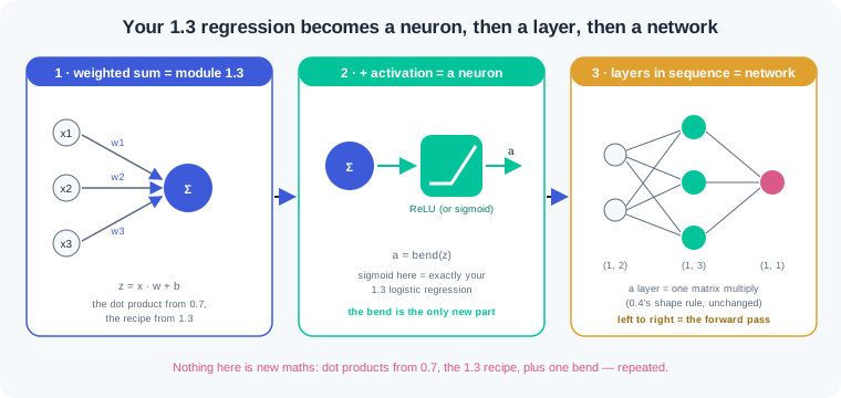
Here is the secret this phase opens with: you already built a neuron in module 1.3. Logistic regression computed a weighted sum of features, then squashed it through the sigmoid. A neuron — a weighted sum of inputs plus a squashing step — is exactly that machine. Same numbers, same code, new name. Deep learning does not replace your regression; it multiplies it.
The squashing step gets its own name now. An activation function — the bending step applied after a neuron's weighted sum — is what makes the neuron more than a line. The sigmoid from 1.3 is one choice. The workhorse today is ReLU — a function that keeps positive values and turns negatives into zero. It costs one comparison, and it gives the network its bend.
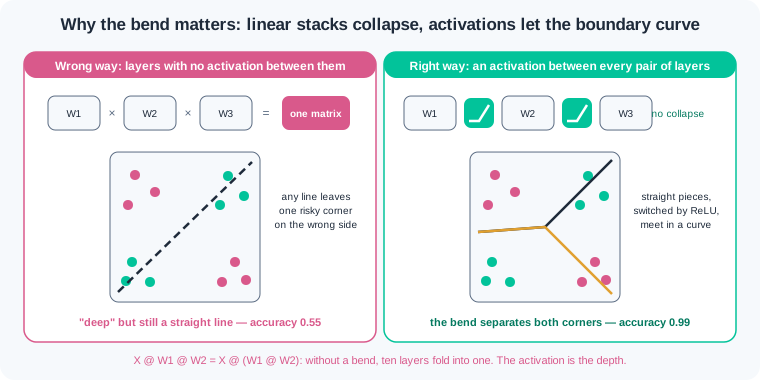
Why does the bend matter so much? Stack two linear layers with no activation between them and the matrices collapse: X @ W1 @ W2 equals X @ (W1 @ W2), which is one matrix. The wrong way stacks ten linear layers and believes depth was added; the algebra quietly folds them into a single line. The right way puts an activation between every pair of layers, so each layer can bend the space before the next one works on it. Bends compose into curves; lines compose into lines.
Now put neurons side by side. A layer is several neurons reading the same input in parallel, and 0.4 already gave you its language: one matrix multiply. An input of shape (1, 2) meets a weight matrix of shape (2, 3) and out comes (1, 3) — three neurons answered at once. A hidden layer — any layer sitting between the input and the final output — is where the network builds its own features. Nobody hand-computes big matrices at work; the skill is predicting every shape before NumPy does.
A network is layers in sequence: the output of one becomes the input of the next. Running data through the whole chain, input to output, is the forward pass — one complete left-to-right trip through the network. That trip is the entire prediction machinery; there is nothing else hiding inside. Training, the part that chooses the weights, waits for module 2.2.
Two pictures from earlier modules survive the jump. The loss landscape from 0.7 is still a surface with a downhill direction; it now lives in thousands of dimensions, one per weight, and the ball still rolls the same way. And on depth against width: a wide single layer must learn every pattern from scratch, while stacked layers reuse work. Early layers make small bends, and later layers combine those bends into shapes. That reuse is why depth wins in practice.
Work inside ai-lab with NumPy only — no frameworks anywhere in this module. Type each block, run it, then change one number and watch what moves.
Step 1 — 1.3's logistic regression, rewritten as a one-neuron network. These are the exact scaled coefficients, intercept, and the silent-95-days customer from the 1.3 watch block:
import numpy as np

w = np.array([-0.82, 2.14, 0.12])   # 1.3's scaled coefficients
b = -1.86                            # 1.3's intercept
x = np.array([-2.06, 1.03, -0.96])  # silent-95-days customer, scaled

z = x @ w + b
p = 1 / (1 + np.exp(-z))
print("weighted sum z :", round(z, 2))
print("after sigmoid p:", round(p, 2))
Output: weighted sum z : 1.92 then after sigmoid p: 0.87. That 0.87 is the same churn probability sklearn printed in 1.3 — dot product from 0.7, sigmoid from 1.3, nothing new. You have been running a one-neuron network for a whole phase. The weighted sum is the neuron's score; the sigmoid is its activation function; w and b are its weights and bias.
Step 2 — the collapse: two linear layers are one matrix. Remove the activation and watch depth vanish:
rng = np.random.default_rng(21)
X = rng.normal(0, 1, (4, 2)).round(2)

W1 = np.array([[2.0, -1.0,  0.5],
               [1.0,  3.0, -2.0]])   # layer 1: 2 -> 3
W2 = np.array([[1.0], [-1.0], [2.0]])  # layer 2: 3 -> 1

deep = (X @ W1) @ W2          # two "layers", no activation
combined = W1 @ W2
flat = X @ combined           # one layer

print("W1 @ W2 =\n", combined)
print("identical outputs:", np.allclose(deep, flat))
Output: the combined matrix prints [[ 4.] [-6.]], then identical outputs: True. Two layers of shapes (2, 3) and (3, 1) folded into a single (2, 1) matrix, exactly as 0.4's shape rule predicts. However many linear layers you stack, the algebra hands back one line. This is why WR-119's network was stuck at logistic-regression accuracy: the builder forgot the activations, so the "deep" model was a straight line wearing a costume.
Step 3 — the forward pass by hand: a 2-3-1 network, every shape and value printed. One input with 2 features, a hidden layer of 3 ReLU neurons, one sigmoid output:
x  = np.array([[2.0, 3.0]])          # shape (1, 2)
W1 = np.array([[0.5, -1.0,  1.0],
               [1.0,  0.5, -1.0]])   # (2, 3)
b1 = np.array([0.0, 1.0, -2.0])
W2 = np.array([[1.0], [-2.0], [0.5]])  # (3, 1)
b2 = np.array([1.0])

z1 = x @ W1 + b1
a1 = np.maximum(0, z1)               # ReLU
z2 = a1 @ W2 + b2
y  = 1 / (1 + np.exp(-z2))           # sigmoid

for name, arr in [("x", x), ("z1", z1), ("a1", a1), ("z2", z2), ("y", y)]:
    print(f"{name:2s} {arr.shape} {arr.round(3)}")
Output, line by line: x (1, 2) [[2. 3.]], z1 (1, 3) [[ 4. 0.5 -3. ]], a1 (1, 3) [[4. 0.5 0. ]], z2 (1, 1) [[4.]], y (1, 1) [[0.982]]. Read it like a story. Three hidden neurons each took a weighted sum of the two inputs: 2×0.5 + 3×1.0 + 0 gives 4.0, and so on across the row. ReLU then kept 4.0 and 0.5 but killed −3.0 to zero — the third neuron stayed silent for this input. The output neuron took a weighted sum of the survivors, 4×1 + 0.5×(−2) + 0×0.5 + 1 = 4.0, and the sigmoid turned it into 0.982. Every deep network you will ever run is this loop with bigger shapes.
Step 4 — ReLU close up: which neurons speak for which input? Same network, two different inputs:
print("before ReLU:", np.array([-3.0, -0.5, 0.0, 0.5, 4.0]))
print("after  ReLU:", np.maximum(0, np.array([-3.0, -0.5, 0.0, 0.5, 4.0])))

for xx in [np.array([[2.0, 3.0]]), np.array([[3.0, 0.5]])]:
    zz = xx @ W1 + b1
    print(xx[0], "-> z1", zz.round(2)[0], "active:", (zz > 0).astype(int)[0])
Output: before ReLU: [-3. -0.5 0. 0.5 4. ], after ReLU: [0. 0. 0. 0.5 4. ], then [2. 3.] -> z1 [ 4. 0.5 -3. ] active: [1 1 0] and [3. 0.5] -> z1 [ 2. -1.75 0.5 ] active: [1 0 1]. ReLU is brutal and cheap: negatives become zero, positives pass untouched. The interesting part is the active pattern — different inputs switch on different neuron subsets, so the network behaves like a different linear model in different regions. That region-by-region switching is precisely how straight pieces assemble into a curved boundary.
Step 5 — a problem no straight line can solve. An XOR-style fraud pattern: risk lives in two opposite corners, like Mounika's mule accounts:
rng = np.random.default_rng(2)
pts = rng.uniform(0, 1, (200, 2)).round(2)          # two scaled features
labels = ((pts[:, 0] > 0.5) != (pts[:, 1] > 0.5)).astype(int)

line_pred = (pts[:, 0] + pts[:, 1] - 1 > 0).astype(int)   # best-effort line
print("straight line accuracy:", (line_pred == labels).mean())
Output: straight line accuracy: 0.545. Rotate the line, shift it, flip it — every straight cut through this square leaves roughly half the points on the wrong side, because the two risky corners sit diagonal to each other. This is the wall Mounika hit, and 1.3's model cannot climb it no matter how well it trains. The failure is geometric, not statistical.
Step 6 — the same problem, solved by a tiny net with hand-set weights. Four ReLU neurons detect the two diagonals; the output layer votes between them:
W1n = np.array([[ 1.0, -1.0,  1.0, -1.0],
                [ 1.0, -1.0, -1.0,  1.0]])   # (2, 4)
b1n = np.array([-1.0, 1.0, 0.0, 0.0])
W2n = np.array([[-1.0], [-1.0], [1.0], [1.0]])  # (4, 1)

a1n = np.maximum(0, pts @ W1n + b1n)
net_pred = ((a1n @ W2n).ravel() > 0).astype(int)
print("tiny net accuracy     :", (net_pred == labels).mean())

no_act = ((pts @ (W1n @ W2n)).ravel() + b1n @ W2n > 0).astype(int)
print("same net, ReLU deleted:", (no_act == labels).mean())
print("collapsed matrix      :", (W1n @ W2n).ravel(), b1n @ W2n)
Output: tiny net accuracy : 0.99, then same net, ReLU deleted: 0.49, then collapsed matrix : [0. 0.] [0.]. The bent boundary took 13 numbers: no training happened, the weights were written by hand, and the forward pass alone scores 0.99 where every line stalls near 0.55. Then the cruel control experiment: delete ReLU and the same weights collapse to the zero matrix — the network predicts nothing and lands at 0.49, a coin flip. The gap between 0.99 and 0.49 is the activation function, and nothing else changed. Module 2.2 teaches the machine to find such weights itself; today you proved the architecture can hold them.
Work inside ai-lab, NumPy only. Every exercise is seeded or fully specified, so where a number is given your output must match it exactly.
The interview classic: forward pass on paper first. A 2-3-1 network with ReLU hidden neurons and a sigmoid output has these weights: W1 = [[1.0, -0.5, 2.0], [0.5, 1.0, -1.0]], b1 = [-1.0, 0.5, 0.0], W2 = [[-1.0], [1.0], [-2.0]], b2 = [0.5]. On paper or a calculator — no NumPy yet — trace two inputs through the full network: [1.0, 2.0] and [2.0, 0.0]. For each, write down z1, a1 after ReLU, z2, and the sigmoid output, plus the shape of every intermediate. Only then create trace_check.py, code the same forward pass, and print every intermediate with its shape to verify your paper numbers. Finish with one comment line naming which hidden neuron was silent for each input. Check: your paper and printed values agree line for line; input [1.0, 2.0] gives z1 [1.0, 2.0, 0.0], z2 [1.5] and output 0.8176; input [2.0, 0.0] gives a1 [1.0, 0.0, 4.0], z2 [-8.5] and output 0.0002; the comment names neuron 3 silent for the first input and neuron 2 for the second.
Build your own layer, then a network from it. Create dense.py with a function dense_layer(x, W, b, activation=None) that returns x @ W + b passed through "relu", "sigmoid", or no activation. Build a 4-5-3-1 network from three calls: draw the input as np.random.default_rng(5).uniform(-1, 1, (8, 4)).round(2), then from the same generator draw W matrices with rng.normal(0, 0.5, shape) for the first two layers and rng.normal(0, 2.0, (3, 1)) for the last, all biases zero. Use ReLU on both hidden layers and sigmoid on the output. Print the shape after every layer, then the output column rounded to 2 decimals and its mean. Last, deliberately call the layers in the wrong order — second layer first — and paste the full error message as a comment. Check: the printed shape sequence is (8, 4), (8, 5), (8, 3), (8, 1); every output value lies strictly between 0 and 1 and the mean prints 0.48; the pasted error says size 5 is different from 4, and a final comment explains that mismatch using 0.4's shape rule.
The activation audit. Create audit.py. Rebuild the step 5 XOR world exactly (seed 2, 200 points, same labels) and the step 6 tiny net with its hand-set weights. Run three versions of the forward pass and print each accuracy with a label: (a) the net as given, (b) the net with every np.maximum deleted, (c) a single layer using the collapsed matrix W1n @ W2n and collapsed bias b1n @ W2n. Also print the collapsed matrix itself. Then write a two-sentence explanation in the file as comments: sentence one states why (b) and (c) print identical accuracy, sentence two states what the collapsed matrix's values reveal about what the "deep" model turned into. Check: the three accuracies print 0.99, 0.49, 0.49; the collapsed matrix prints as zeros; version (b) and (c) agree on every single prediction, which you verify with an np.array_equal print; your sentences name the collapse (linear stacks fold into one matrix) and note that this particular fold is the zero function, which predicts one class for everything.
Three first-network failures cover most of the pain in this module. Each has a War Room entry with the full diagnosis path:
- WR-118 — the shape mismatch five layers deep. A matmul between (32, 10) and (3, 1) exploded mid-network and the error pointed nowhere useful; the fix is 0.4's reflex scaled up — print every layer's output shape before trusting the chain.
- WR-119 — the network that could only draw straight lines. Activations were forgotten between layers, so a five-layer model collapsed to one matrix and sat exactly at logistic-regression accuracy; the fix is the collapse demo plus an activation audit of every layer.
- WR-120 — the exploding forward pass. Weights initialised too large multiplied values into
infwithin three layers; the fix is small random initialisation and watching the magnitude of each layer's output.
A neuron is the machine you built in module 1.3: a weighted sum of inputs followed by an activation function. Without that bending step, stacked layers collapse into a single matrix, so a deep linear network is one line in disguise. ReLU supplies the bend cheaply by zeroing negatives, and different inputs switch on different neurons, letting straight pieces assemble into curves. A layer is neurons in parallel via one matrix multiply, a network is layers in sequence, and the forward pass is one full trip through them. The loss surface now has thousands of dimensions, but the downhill picture from module 0.7 still holds, and module 2.2 starts rolling the ball.
- UPI fraud engines at Indian payment firms score each transaction with stacked layers, because mule-account patterns sit in opposite corners of the feature space where no single line can cut.
- Quick-commerce logistics teams feed order, rider, and weather features through small dense networks for delivery-time prediction when the straight-line model from 1.3 plateaus.
- Every LLM you will use in Phase 3 is this module's forward pass at scale: weighted sums, activations, layer after layer — billions of weights, same trip.
Answer these before opening the gate assessment. Each question names its type.
type=output-prediction— A 2-2-1 network hasW1 = [[1, 0], [0, 1]],b1 = [-2, 0], ReLU, thenW2 = [[1], [1]],b2 = 0. For input[1, 2], predict whata1and the final output print, showing the one-line arithmetic for each.type=debug— A teammate's five-layer script dies withmatmul: size 3 is different from 10and they are editing layer one. Name the single print statement you would add through the network, and state what the mismatched pair of numbers tells you about where the wrong matrix lives.type=interpretation— A forward-pass log showsz1 = [2.1, -0.7, 0.4]anda1 = [2.1, 0.0, 0.4]. Explain what happened to the second neuron, and what it means for how this network treats this particular input.type=scenario-judgement— A teammate proposes a ten-layer network with no activations "to keep it fast", claiming depth alone adds power. Give your judgement, the one-line matrix argument that settles it, and the accuracy you expect relative to logistic regression.type=trade-off— Compare one very wide hidden layer against several narrower stacked layers for a bent-boundary problem. Give one concrete advantage and one concrete cost of each choice, and name what the stacked version can reuse that the wide one cannot.
Explain to a friend who finished module 1.3 but fears deep learning: how is the churn model they already built secretly one neuron, and why does adding a bend between stacked layers let the model draw curves that no straight line can? Use at most 4 sentences and no maths symbols beyond "multiply and add". If your friend says "so it is my regression, repeated", you own this module.