RNN to LSTM to why attention won
Shalini sorts customer reviews at a bus-ticketing company in Davangere. Her word-count model tags each review as happy or angry, and the weekly report looked fine. Then a rider wrote that the app was good and the refund was not slow. The model called it angry. Her lead circled two words on the screen. "Your model counted the word not and the word slow," she said. "It never saw which one came first." Tonight Shalini builds a model that reads in order.
- "Why did attention replace RNNs?" is asked in almost every Indian AI interview that touches language, and tonight your answer is a measured table rather than a story you repeat.
- Every model in Phase 3 sits on top of attention. You will read RAG code, LLM code and agent code with far less fear once you have computed attention weights with your own hands on four tokens.
- The whole module is CPU-only on an 8GB laptop. The longest run below takes about 36 seconds, and every number printed here came from that machine.
Module 1.6 turned text into counts, and 2.6 turned photos into features. Counting words works well until the order carries the meaning. "delivery was good and service was not slow" and "delivery was slow and service was not good" hold exactly the same eight words. One review is a compliment and the other is a complaint. A model that only counts words sees one bag, and it must give both the same answer.
There is a wrong way and a right way to read a review. The wrong way pours the words into a bag and counts them, so the word "not" floats free of the word it changes. On this module's data that model scores 1.000 on rows with no negation and 0.485 on rows that carry "not", which is a coin toss. The right way reads the words in order and keeps a small memory while it reads. The same model family, reading the same rows in order, scores 1.000 on both halves.
A sequence model — any model that reads its input one step at a time and keeps state between steps — is the fix. The plainest one is the recurrent neural network, a network that applies the same small function to every step of the input. It carries a hidden state — a short vector of numbers holding what the model has read so far. Each step mixes the new token with the old state and writes a new state, and one line holds the whole idea.
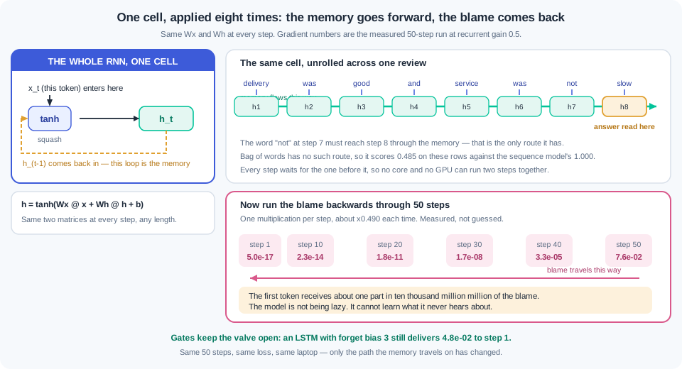
Reading step by step has a price, and you will measure it rather than believe it. Blame has to travel back down the chain, one multiplication per step. Multiply by a number below one fifty times over and almost nothing arrives. That is the vanishing gradient — the blame signal shrinking toward zero as it travels back through many steps. In the table below, the blame at step 50 reads 7.577e-02 while the blame at step 1 reads 5.032e-17.
Push the same knob the other way and the mirror problem appears. With a slightly larger recurrent weight, the blame at step 1 reads 5.271e+00, which is 68 times the blame at step 50. Huge steps follow, the loss turns to nan, and teams reach for gradient clipping. Both faults come from the same place: one shared matrix, applied over and over. A plain RNN forgets the start of a long review, and that is a property of its design, not a bug in your code.
Gates were engineered to fix the forgetting. A gate — a number between 0 and 1 that decides how much of a signal passes — behaves like a valve on a pipe. An LSTM keeps a separate cell state and puts three valves on it: forget, input and output. The forget valve decides what stays, the input valve decides what enters, and the output valve decides what is read out. While the forget valve stays open the memory flows through untouched, and so does the blame.
The measured effect is large, and it only shows up at length. On a recall task of 50 steps, a plain RNN scores 0.507 on held-back rows while an LSTM with open forget gates scores 1.000. At 5 steps and at 20 steps every model scores 1.000, so length is the whole story here. A GRU is the same idea with two valves instead of three and fewer weights, and it often matches the LSTM.
Gates buy memory, and they buy no speed at all. A recurrent layer must finish step 49 before it can start step 50, so the work cannot be spread across cores or across a GPU. One LSTM pass over 1000 steps takes 66.6 ms on this laptop, while an attention pass over the same input takes 32.1 ms. Long links also stay fragile, because the path from token 1 to token 50 is still 49 hops through the same squashing function.
Attention — letting every position read every other position directly, in one parallel pass — removes both problems at once. Each position sends out a query, every position answers with a key, and the match scores become weights through a softmax. Those weights then mix the value vectors into a fresh meaning for that position. The path between any two tokens drops from 49 hops to 1 hop. Module 0.7 called the dot product a similarity score, and that is exactly the job it does here on 3.4's embeddings.
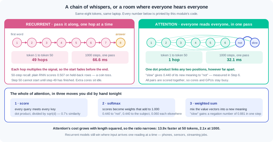
Be honest about the history, because interviewers ask about it. This module is the reason the Transformer exists, and 2.8 builds one block by block. RNNs did not disappear. They still run on tiny devices, in streaming jobs where one reading arrives at a time, and in places where one small matrix per step is cheaper than comparing every pair. They also live on in interviews, because the vanishing-gradient story is the cleanest test of whether a candidate understands training.
Work inside ai-lab with torch and numpy. One-time setup: pip install torch==2.9.* numpy==2.5.* — the CPU build is all this course needs, and no dataset is downloaded anywhere in this module. Every sequence here is generated in code, so the whole lesson runs offline on an 8GB laptop with no GPU. Timings below come from a plain CPU laptop with four threads; the accuracies are seeded and should land within about 1% of the printed ones — seeded torch runs vary slightly across builds.
If your numbers are close but not identical, triage in a fixed order before touching your code. Everything off by a little — every value drifting in the last decimal or two — points at a library version: run pip show torch, compare it with the pinned install line above, and match the pin, because the printed numbers were produced on that version. One number wildly off while the rest agree points at stale state: restart from a fresh kernel or a fresh python and run the file top to bottom, since seeded draws only reproduce when they happen in the same order from a clean start. Only when both checks pass and the numbers still disagree should you suspect your own logic — diff your script line by line against the printed code.
Step 1 — the shared world, and the failure that starts the module. Save this as sequences.py; every later step imports it:
import time, numpy as np, torch, torch.nn as nn

torch.set_num_threads(4)

SUBJECTS = ["delivery", "service", "packing", "app", "support"]
POS = ["good", "quick", "clean", "helpful"]
NEG = ["bad", "slow", "dirty", "rude"]
VOCAB = SUBJECTS + POS + NEG + ["was", "and", "very", "not"]
STOI = {w: i for i, w in enumerate(VOCAB)}


def make_reviews(n, seed):
    """Eight-token reviews. One clause carries 'very' or 'not', either clause."""
    rng = np.random.default_rng(seed)
    rows = []
    for _ in range(n):
        s1, s2 = rng.choice(SUBJECTS, 2, replace=False)
        pol = int(rng.random() < 0.5)                 # 1 = positive review
        mod = "very" if rng.random() < 0.5 else "not"
        plain_pool = POS if pol else NEG              # the clause with no modifier
        mod_pool = plain_pool if mod == "very" else (NEG if pol else POS)
        if rng.random() < 0.5:                        # modifier on clause one
            toks = [s1, "was", mod, str(rng.choice(mod_pool)), "and",
                    s2, "was", str(rng.choice(plain_pool))]
        else:                                         # modifier on clause two
            toks = [s1, "was", str(rng.choice(plain_pool)), "and",
                    s2, "was", mod, str(rng.choice(mod_pool))]
        rows.append((toks, pol, mod))
    return rows


def encode(rows):
    X = torch.tensor([[STOI[w] for w in toks] for toks, _, _ in rows])
    y = torch.tensor([lab for _, lab, _ in rows], dtype=torch.float32)
    return X, y, np.array([k for _, _, k in rows])


def bag(X):
    """Bag of words: how many times each word appears. Order thrown away."""
    B = torch.zeros(len(X), len(VOCAB))
    for i, row in enumerate(X):
        for t in row:
            B[i, int(t)] += 1.0
    return B


loss_fn = nn.BCEWithLogitsLoss()


def train(net, X, y, epochs=30, lr=0.01, bs=64, seed=7):
    torch.manual_seed(seed)
    opt = torch.optim.Adam(net.parameters(), lr=lr)
    g = torch.Generator().manual_seed(seed)
    for _ in range(epochs):
        net.train()
        for i in torch.randperm(len(X), generator=g).split(bs):
            opt.zero_grad()                            # 2.3's five steps, unchanged
            loss_fn(net(X[i]).squeeze(-1), y[i]).backward()
            opt.step()
    return net


@torch.no_grad()
def acc(net, X, y, mask=None):
    net.eval()
    ok = ((net(X).squeeze(-1) > 0).float() == y).float()
    return float(ok.mean()) if mask is None else float(ok[mask].mean())
Now the demonstration itself, in step1_order.py:
import torch, torch.nn as nn
from sequences import *

Xtr, ytr, ktr = encode(make_reviews(1600, seed=11))
Xte, yte, kte = encode(make_reviews(600, seed=12))
very, nots = torch.tensor(kte == "very"), torch.tensor(kte == "not")

print(f"vocabulary {len(VOCAB)} words; every review is {Xtr.shape[1]} tokens")
print(f"train {tuple(Xtr.shape)}   test {tuple(Xte.shape)}"
      f"   test rows: {int(very.sum())} 'very', {int(nots.sum())} 'not'")
for toks, lab, kind in make_reviews(4, seed=12):
    print(f"  {' '.join(toks):<52s} label {lab}  ({kind})")

a = ["delivery", "was", "good", "and", "service", "was", "not", "slow"]
b = ["delivery", "was", "slow", "and", "service", "was", "not", "good"]
print(f"\ntwin A -> positive: {' '.join(a)}")
print(f"twin B -> negative: {' '.join(b)}")
print("A sorted:", sorted(a))
print("B sorted:", sorted(b))
print("same multiset of words?", sorted(a) == sorted(b))
ba = bag(torch.tensor([[STOI[w] for w in a]]))
bb = bag(torch.tensor([[STOI[w] for w in b]]))
print("same bag-of-words vector? ", bool(torch.equal(ba, bb)))

Btr, Bte = bag(Xtr), bag(Xte)
print(f"\nbag-of-words matrix {tuple(Btr.shape)} — order is gone for good")
print(f"\n{'model (order thrown away)':<28s} {'params':>7s} {'all':>7s}"
      f" {'very rows':>10s} {'not rows':>9s}")
for name, build in (("logistic on word counts", lambda: nn.Linear(len(VOCAB), 1)),
                    ("64-unit net on counts",
                     lambda: nn.Sequential(nn.Linear(len(VOCAB), 64), nn.ReLU(),
                                           nn.Linear(64, 1)))):
    torch.manual_seed(7)                        # seed BEFORE the weights are made
    net = build()
    train(net, Btr, ytr, epochs=60, lr=0.01)
    print(f"{name:<28s} {sum(p.numel() for p in net.parameters()):7,d}"
          f" {acc(net, Bte, yte):7.3f} {acc(net, Bte, yte, very):10.3f}"
          f" {acc(net, Bte, yte, nots):9.3f}")

scores = []                                     # one test set is one exam
for s in range(12, 32):
    X, y, k = encode(make_reviews(600, seed=s))
    scores.append(acc(net, bag(X), y, torch.tensor(k == "not")))
print(f"\nthe 64-unit model's 'not' score on 20 fresh test sets:")
print(f"  min {min(scores):.3f}   mean {sum(scores) / len(scores):.3f}"
      f"   max {max(scores):.3f}")
Output:
vocabulary 17 words; every review is 8 tokens
train (1600, 8)   test (600, 8)   test rows: 297 'very', 303 'not'
  packing was very helpful and service was quick       label 1  (very)
  delivery was helpful and support was not bad         label 1  (not)
  packing was very good and service was helpful        label 1  (very)
  service was clean and app was very helpful           label 1  (very)

twin A -> positive: delivery was good and service was not slow
twin B -> negative: delivery was slow and service was not good
A sorted: ['and', 'delivery', 'good', 'not', 'service', 'slow', 'was', 'was']
B sorted: ['and', 'delivery', 'good', 'not', 'service', 'slow', 'was', 'was']
same multiset of words? True
same bag-of-words vector?  True

bag-of-words matrix (1600, 17) — order is gone for good

model (order thrown away)     params     all  very rows  not rows
logistic on word counts           18   0.740      1.000     0.485
64-unit net on counts          1,217   0.785      1.000     0.574

the 64-unit model's 'not' score on 20 fresh test sets:
  min 0.448   mean 0.504   max 0.574
Read the twin pair first, because it is the argument of the whole module. Both reviews contain and, delivery, good, not, service, slow, was, was and nothing else, so their bag-of-words rows are byte-for-byte identical, yet one is positive and the other is negative. No model reading that bag can score above 0.500 on such rows, whatever its size. The table proves it: logistic regression reads 1.000 on the "very" rows, where counting really is enough, and 0.485 on the "not" rows. Growing the model from 18 weights to 1,217 appears to help, lifting the "not" column to 0.574, and the last two lines are there to stop you believing it. The same trained model scored between 0.448 and 0.574 across 20 freshly generated test sets, averaging 0.504 — so 0.574 was one lucky exam on 303 rows, and 1.8's warning about a single split applies to text exactly as it did to tables. The overall 0.740 is the number that gets shipped and the number that lies, an average across a half that works perfectly and a half that is random. Split your accuracy by row type before you trust it, which is 1.5's habit applied to text.
Step 2 — the RNN loop, in NumPy, with the memory printed at every step. Hand-set weights, so you can read what the memory holds:
import numpy as np
from sequences import POS, NEG

np.set_printoptions(precision=3, suppress=True)

def features(tok):
    """Three input numbers per token: positive, negative, or the word 'not'."""
    return np.array([float(tok in POS), float(tok in NEG), float(tok == "not")])

Wx = np.array([[0.9, -0.9, 0.0],      # h1: running mood
               [0.0, 0.0, 2.0],       # h2: did I just read the word "not"
               [0.5, 0.5, 0.0]])      # h3: how many opinion words so far
Wh = np.array([[1.0, 0.0, 0.0],       # h1 carries itself forward
               [0.0, 0.0, 0.0],       # h2 forgets everything each step
               [0.0, 0.0, 1.0]])      # h3 carries itself forward
b = np.zeros(3)

def run_rnn(tokens, show=False):
    h = np.zeros(3)                                   # the memory starts empty
    if show:
        print(f"{'step':>4s} {'token':<10s} {'x_t (pos,neg,not)':<20s}"
              f" {'h_t (mood, saw-not, count)':<28s}")
        print(f"{0:4d} {'<start>':<10s} {str(np.zeros(3)):<20s} {str(h):<28s}")
    for t, tok in enumerate(tokens, start=1):
        x = features(tok)
        h = np.tanh(Wx @ x + Wh @ h + b)              # the whole RNN, one line
        if show:
            print(f"{t:4d} {tok:<10s} {str(x):<20s} {str(h):<28s}")
    return h

A = ["delivery", "was", "good", "and", "service", "was", "not", "slow"]
B = ["delivery", "was", "slow", "and", "service", "was", "not", "good"]

print("REVIEW A  (positive):", " ".join(A))
hA = run_rnn(A, show=True)
print("\nREVIEW B  (negative):", " ".join(B))
hB = run_rnn(B, show=True)

print(f"\nfinal memory A: {hA}")
print(f"final memory B: {hB}")
print(f"they differ by : {np.abs(hA - hB).max():.3f}  <- order changed the memory")

bagA, bagB = sum(features(t) for t in A), sum(features(t) for t in B)
print(f"\nthe same features summed, order thrown away")
print(f"  A: {bagA}\n  B: {bagB}\n  identical? {np.array_equal(bagA, bagB)}")

print("\nsame 8 words, 3 orders, one RNN:")
for label, seq in (("as written  ", A), ("reversed    ", A[::-1]),
                   ("shuffled    ", [A[i] for i in [4, 0, 7, 2, 6, 1, 5, 3]])):
    h = run_rnn(seq)
    print(f"  {label} mood {h[0]:+.3f}   count {h[2]:.3f}   {' '.join(seq)}")
Output:
REVIEW A  (positive): delivery was good and service was not slow
step token      x_t (pos,neg,not)    h_t (mood, saw-not, count)
   0 <start>    [0. 0. 0.]           [0. 0. 0.]
   1 delivery   [0. 0. 0.]           [0. 0. 0.]
   2 was        [0. 0. 0.]           [0. 0. 0.]
   3 good       [1. 0. 0.]           [0.716 0.    0.462]
   4 and        [0. 0. 0.]           [0.615 0.    0.432]
   5 service    [0. 0. 0.]           [0.547 0.    0.407]
   6 was        [0. 0. 0.]           [0.499 0.    0.386]
   7 not        [0. 0. 1.]           [0.461 0.964 0.368]
   8 slow       [0. 1. 0.]           [-0.413  0.     0.7  ]

REVIEW B  (negative): delivery was slow and service was not good
step token      x_t (pos,neg,not)    h_t (mood, saw-not, count)
   0 <start>    [0. 0. 0.]           [0. 0. 0.]
   1 delivery   [0. 0. 0.]           [0. 0. 0.]
   2 was        [0. 0. 0.]           [0. 0. 0.]
   3 slow       [0. 1. 0.]           [-0.716  0.     0.462]
   4 and        [0. 0. 0.]           [-0.615  0.     0.432]
   5 service    [0. 0. 0.]           [-0.547  0.     0.407]
   6 was        [0. 0. 0.]           [-0.499  0.     0.386]
   7 not        [0. 0. 1.]           [-0.461  0.964  0.368]
   8 good       [1. 0. 0.]           [0.413 0.    0.7  ]

final memory A: [-0.413  0.     0.7  ]
final memory B: [0.413 0.    0.7  ]
they differ by : 0.826  <- order changed the memory

the same features summed, order thrown away
  A: [1. 1. 1.]
  B: [1. 1. 1.]
  identical? True

same 8 words, 3 orders, one RNN:
  as written   mood -0.413   count 0.700   delivery was good and service was not slow
  reversed     mood +0.372   count 0.540   slow not was service and good was delivery
  shuffled     mood +0.174   count 0.468   service delivery slow good not was was and
Five things to notice, and the first is the loop itself. The entire recurrent network is one line, h = np.tanh(Wx @ x + Wh @ h + b), run once per token, with the same Wx and Wh every time — that weight sharing is what lets one small model read a sequence of any length. Second, the memory column: unit 1 rises to 0.716 when "good" arrives and stays near it while filler words pass, which is memory you can watch. Third, unit 2 was built to forget: its row of Wh is all zeros, so it reads 0.964 at the "not" step and drops back to 0.000 at the next step, and that one-step memory is exactly what a real gate learns to hold open longer. Fourth, unit 1 also fades on its own — 0.716, 0.615, 0.547, 0.499 — with no new evidence at all, because tanh squashes a little more at every pass, and that fade is the vanishing gradient wearing its forward-facing clothes. Fifth, the comparison that closes step 1: the summed features for A and B are the identical [1. 1. 1.], while the RNN's final memories differ by 0.826, and the three orderings of the same eight words give three different answers.
Step 3 — the vanishing gradient, measured rather than described. One 50-step sequence, a loss only at the last step, and a printed record of how much blame arrives at each earlier step:
import torch, torch.nn as nn

torch.manual_seed(0)
T, H, D, B = 50, 32, 16, 64
x = torch.randn(T, B, D) * 0.5                  # 64 sequences, 50 steps each
v = torch.randn(H, 1) * 0.2                     # read-out at the LAST step only
y = torch.ones(B, 1)


def rnn_grads(gain):
    """Plain RNN. Gradient norm arriving at each step's hidden state."""
    torch.manual_seed(1)
    Wx = (torch.randn(D, H) * 0.1).requires_grad_()
    Wh = (torch.randn(H, H) / H ** 0.5 * gain).requires_grad_()
    h, hs = torch.zeros(B, H), []
    for t in range(T):
        h = torch.tanh(x[t] @ Wx + h @ Wh)
        h.retain_grad(); hs.append(h)           # keep every step's gradient
    nn.functional.binary_cross_entropy_with_logits(hs[-1] @ v, y).backward()
    return [float(h.grad.norm()) for h in hs]


def lstm_grads(forget_bias):
    """LSTM. Gradient norm arriving at each step's CELL state."""
    torch.manual_seed(1)
    cell = nn.LSTMCell(D, H)
    with torch.no_grad():                       # start the forget valve open
        cell.bias_ih[H:2 * H].fill_(forget_bias)
        cell.bias_hh[H:2 * H].fill_(0.0)
    h, c, cs = torch.zeros(B, H), torch.zeros(B, H), []
    for t in range(T):
        h, c = cell(x[t], (h, c))
        c.retain_grad(); cs.append(c)
    nn.functional.binary_cross_entropy_with_logits(h @ v, y).backward()
    return [float(c.grad.norm()) for c in cs]


cols = {"RNN gain 0.5": rnn_grads(0.5), "RNN gain 1.0": rnn_grads(1.0),
        "RNN gain 1.5": rnn_grads(1.5), "LSTM b_f=0": lstm_grads(0.0),
        "LSTM b_f=3": lstm_grads(3.0)}

print("Blame reaching step t when the only loss sits at step 50")
print(f"{'step':>5s}" + "".join(f"{k:>14s}" for k in cols))
for t in [50, 45, 40, 30, 20, 10, 5, 1]:
    print(f"{t:5d}" + "".join(f"{c[t - 1]:14.3e}" for c in cols.values()))

print(f"\n{'model':<14s} {'step 50':>12s} {'step 1':>12s} {'step1/step50':>13s}"
      f"  {'shrinks per step':>16s}")
for k, c in cols.items():
    r = (c[0] / c[-1]) ** (1 / (T - 1))
    print(f"{k:<14s} {c[-1]:12.3e} {c[0]:12.3e} {c[0] / c[-1]:13.2e}"
          f"  {'x' + format(r, '.3f'):>16s}")
Output:
Blame reaching step t when the only loss sits at step 50
 step  RNN gain 0.5  RNN gain 1.0  RNN gain 1.5    LSTM b_f=0    LSTM b_f=3
   50     7.577e-02     7.603e-02     7.708e-02     3.679e-02     2.230e-02
   45     1.331e-03     2.923e-02     6.957e-02     2.117e-03     1.890e-02
   40     3.256e-05     1.459e-02     7.066e-02     1.824e-04     1.728e-02
   30     1.732e-08     4.252e-03     9.759e-02     1.869e-06     1.772e-02
   20     1.787e-11     1.962e-03     2.421e-01     2.514e-08     2.136e-02
   10     2.281e-14     1.140e-03     8.056e-01     3.026e-10     2.873e-02
    5     7.499e-16     9.106e-04     1.629e+00     3.158e-11     3.699e-02
    1     5.032e-17     7.716e-04     5.271e+00     5.180e-12     4.782e-02

model               step 50       step 1  step1/step50  shrinks per step
RNN gain 0.5      7.577e-02    5.032e-17      6.64e-16            x0.490
RNN gain 1.0      7.603e-02    7.716e-04      1.01e-02            x0.911
RNN gain 1.5      7.708e-02    5.271e+00      6.84e+01            x1.090
LSTM b_f=0        3.679e-02    5.180e-12      1.41e-10            x0.629
LSTM b_f=3        2.230e-02    4.782e-02      2.14e+00            x1.016
This table is the module's centre, so read all five columns. Column one is the textbook picture: a recurrent matrix scaled to gain 0.5 multiplies the blame by about 0.490 per step, so step 1 receives 5.032e-17 against step 50's 7.577e-02 — sixteen orders of magnitude gone, and the first token might as well not exist. Column three is the mirror fault at gain 1.5: blame grows by about 1.090 per step until step 1 receives 5.271e+00, which is 68 times the loss's own gradient, and that is the run that ends in nan and sends people looking for clip_grad_norm_. Column two, the ordinary initialisation, sits in between and still loses 99 percent of the signal over 50 steps, which is why "it trains, but it ignores the beginning" is the usual real-world symptom rather than a crash. Now the two LSTM columns, and note that these track the cell state, the highway the gates protect. With the forget bias left at 0 the valves sit half open, the cell decays by about 0.629 per step, and the LSTM is no better than the RNN — the architecture alone did not save it. Push the forget bias to 3 and the valves start wide open: blame changes by about 1.016 per step and step 1 still receives 4.782e-02, more than step 50 itself. That single initialisation is why so many production LSTM recipes set the forget bias to 1 or higher, and step 5 shows what it is worth in accuracy.
Step 4 — sequence models on the review task, against the bag. Same 1,600 reviews, same split, one honest clock:
import time, torch, torch.nn as nn
from sequences import *


class SeqNet(nn.Module):
    """Embed each word, run one recurrent layer, read the last memory."""

    def __init__(self, kind="lstm", emb=16, hid=32):
        super().__init__()
        self.embed = nn.Embedding(len(VOCAB), emb)       # 3.4's idea, learned here
        core = {"rnn": nn.RNN, "lstm": nn.LSTM, "gru": nn.GRU}[kind]
        self.core = core(emb, hid, batch_first=True)
        self.head = nn.Linear(hid, 1)

    def forward(self, x):
        out, _ = self.core(self.embed(x))
        return self.head(out[:, -1, :])                  # memory after the last word


class BagNet(nn.Module):
    def __init__(self, hid=None):
        super().__init__()
        self.net = (nn.Linear(len(VOCAB), 1) if hid is None else
                    nn.Sequential(nn.Linear(len(VOCAB), hid), nn.ReLU(),
                                  nn.Linear(hid, 1)))

    def forward(self, x):
        return self.net(bag(x))


Xtr, ytr, ktr = encode(make_reviews(1600, seed=11))
Xte, yte, kte = encode(make_reviews(600, seed=12))
very, nots = torch.tensor(kte == "very"), torch.tensor(kte == "not")

print(f"{'model':<24s} {'params':>8s} {'train s':>8s} {'all':>7s}"
      f" {'very':>7s} {'not':>7s}")
for name, build in (("bag of words, logistic", lambda: BagNet()),
                    ("bag of words, 64-unit", lambda: BagNet(64)),
                    ("plain RNN, 32 units", lambda: SeqNet("rnn")),
                    ("GRU, 32 units", lambda: SeqNet("gru")),
                    ("LSTM, 32 units", lambda: SeqNet("lstm"))):
    torch.manual_seed(7)
    net = build()
    t0 = time.perf_counter()
    train(net, Xtr, ytr, epochs=30, lr=0.01)
    dt = time.perf_counter() - t0
    print(f"{name:<24s} {sum(p.numel() for p in net.parameters()):8,d} {dt:8.1f}"
          f" {acc(net, Xte, yte):7.3f} {acc(net, Xte, yte, very):7.3f}"
          f" {acc(net, Xte, yte, nots):7.3f}")
    if name.startswith("LSTM"):
        best = net

pair = [["delivery", "was", "good", "and", "service", "was", "not", "slow"],
        ["delivery", "was", "slow", "and", "service", "was", "not", "good"],
        ["delivery", "was", "not", "good", "and", "service", "was", "slow"],
        ["delivery", "was", "very", "good", "and", "service", "was", "helpful"]]
P = torch.tensor([[STOI[w] for w in s] for s in pair])
with torch.no_grad():
    prob = torch.sigmoid(best(P).squeeze(-1))
print("\nthe trained LSTM on four hand-written reviews:")
for s, p in zip(pair, prob):
    print(f"  P(positive) {float(p):.3f}   {' '.join(s)}")
Output:
model                      params  train s     all    very     not
bag of words, logistic         18      1.4   0.745   1.000   0.495
bag of words, 64-unit       1,217      1.2   0.758   1.000   0.521
plain RNN, 32 units         1,905      0.3   1.000   1.000   1.000
GRU, 32 units               5,105      0.5   1.000   1.000   1.000
LSTM, 32 units              6,705      0.6   1.000   1.000   1.000

the trained LSTM on four hand-written reviews:
  P(positive) 1.000   delivery was good and service was not slow
  P(positive) 0.000   delivery was slow and service was not good
  P(positive) 0.000   delivery was not good and service was slow
  P(positive) 1.000   delivery was very good and service was helpful
Two readings here, and the second one is the honest part that most tutorials leave out. First the win: reading in order takes the "not" column from 0.495 to 1.000, and the four hand-written reviews show what the model learned — it puts 1.000 on the twin that means good and 0.000 on the twin built from the same eight words, and it handles "not" in either clause. That is a real capability that no amount of counting could buy. Second, and say this out loud: the plain RNN also scores 1.000, in 0.3 seconds, with 1,905 parameters, while the LSTM needs 6,705 parameters and twice the time to reach the same score. On eight tokens there is nothing for gates to fix, because the blame only travels seven steps. Choosing an LSTM here would be paying for memory you do not need, and 2.4's lesson applies unchanged — measure before you upgrade. The next step builds the task where the choice actually matters.
Step 5 — memory length, and the wall that RNNs hit. Remember the first token, answer after T-1 meaningless tokens, at three lengths:
import time, torch, torch.nn as nn

torch.set_num_threads(4)
FLAGS, FILLERS = 2, 8            # tokens 0,1 = the flag; tokens 2..9 = noise


def recall_task(n, T, seed):
    """Remember the FIRST token, answer after T-1 meaningless tokens."""
    g = torch.Generator().manual_seed(seed)
    flag = torch.randint(0, FLAGS, (n,), generator=g)
    noise = torch.randint(FLAGS, FLAGS + FILLERS, (n, T - 1), generator=g)
    return torch.cat([flag.unsqueeze(1), noise], 1), flag.float()


class Recaller(nn.Module):
    def __init__(self, kind, hid=32, forget_bias=0.0):
        super().__init__()
        self.embed = nn.Embedding(FLAGS + FILLERS, 16)
        self.core = {"RNN": nn.RNN, "LSTM": nn.LSTM}[kind](16, hid, batch_first=True)
        if forget_bias:                       # start every forget valve wide open
            with torch.no_grad():
                self.core.bias_ih_l0[hid:2 * hid].fill_(forget_bias)
                self.core.bias_hh_l0[hid:2 * hid].fill_(0.0)
        self.head = nn.Linear(hid, 1)

    def forward(self, x):
        out, _ = self.core(self.embed(x))
        return self.head(out[:, -1, :]).squeeze(-1)


loss_fn = nn.BCEWithLogitsLoss()
MODELS = [("RNN", "RNN", 0.0), ("LSTM", "LSTM", 0.0), ("LSTM b_f=3", "LSTM", 3.0)]
print(f"{'length':>7s} {'model':<11s} {'train s':>8s} {'train acc':>10s}"
      f" {'test acc':>9s}")
for T in (5, 20, 50):
    Xtr, ytr = recall_task(4000, T, seed=100 + T)
    Xte, yte = recall_task(1000, T, seed=200 + T)
    for label, kind, fb in MODELS:
        torch.manual_seed(7)
        net = Recaller(kind, forget_bias=fb)
        opt = torch.optim.Adam(net.parameters(), lr=0.01)
        g = torch.Generator().manual_seed(7)
        t0 = time.perf_counter()
        for _ in range(40):
            net.train()
            for i in torch.randperm(len(Xtr), generator=g).split(64):
                opt.zero_grad()
                loss_fn(net(Xtr[i]), ytr[i]).backward()
                nn.utils.clip_grad_norm_(net.parameters(), 1.0)   # for gain 1.5 runs
                opt.step()
        dt = time.perf_counter() - t0
        net.eval()
        with torch.no_grad():
            tr = float(((net(Xtr) > 0).float() == ytr).float().mean())
            te = float(((net(Xte) > 0).float() == yte).float().mean())
        print(f"{T:7d} {label:<11s} {dt:8.1f} {tr:10.3f} {te:9.3f}")

print("\nOne forward pass, batch 32, 128 features: step by step, or all at once")
print(f"{'length':>7s} {'LSTM (sequential)':>19s} {'attention (parallel)':>21s}"
      f" {'ratio':>7s}")
H = 128
lstm = nn.LSTM(H, H, batch_first=True)
for T in (50, 200, 500, 1000):
    x = torch.randn(32, T, H)
    with torch.no_grad():
        lstm(x[:, :8]); (x @ x.transpose(1, 2))                  # warm up
        t0 = time.perf_counter()
        for _ in range(3):
            lstm(x)
        a = (time.perf_counter() - t0) / 3
        t0 = time.perf_counter()
        for _ in range(3):
            torch.softmax(x @ x.transpose(1, 2) / H ** 0.5, -1) @ x
        b = (time.perf_counter() - t0) / 3
    print(f"{T:7d} {a * 1000:16.1f} ms {b * 1000:18.1f} ms {a / b:6.1f}x")
Output:
 length model        train s  train acc  test acc
      5 RNN              0.9      1.000     1.000
      5 LSTM             1.5      1.000     1.000
      5 LSTM b_f=3       1.5      1.000     1.000
     20 RNN              1.8      1.000     1.000
     20 LSTM             4.1      1.000     1.000
     20 LSTM b_f=3       4.1      1.000     1.000
     50 RNN              3.8      0.539     0.507
     50 LSTM             9.2      0.858     0.506
     50 LSTM b_f=3       9.2      1.000     1.000

One forward pass, batch 32, 128 features: step by step, or all at once
 length   LSTM (sequential)  attention (parallel)   ratio
     50              3.3 ms                0.2 ms   13.9x
    200             13.2 ms                1.3 ms   10.4x
    500             33.1 ms                7.6 ms    4.4x
   1000             66.5 ms               30.6 ms    2.2x
The whole block takes about 36 seconds and it earns every one of them. Read the accuracy table down the length column: at 5 steps and at 20 steps all three models are perfect, so anyone benchmarking on short sequences would conclude the choice does not matter. At 50 steps the plain RNN reads 0.507 on held-back rows, which is a coin toss on a task with a single relevant token, and its training accuracy of 0.539 says it never learned the rule at all rather than overfitting it. The plain LSTM row is the trap: 0.858 on training and 0.506 on test, so it memorised 4,000 sequences without discovering the rule, and a teammate who reports only the training number will tell you the LSTM works. Set the forget bias to 3 and the same LSTM reads 1.000 and 1.000 — the architecture needed its gates opened, exactly as step 3's gradient column predicted. Then the timing table, which is why this whole family lost. The LSTM must walk 1000 steps in order and takes 66.6 ms; the attention computation touches every pair at once in 32.1 ms on four CPU threads, and on a GPU with thousands of cores that gap widens enormously. Note the ratio column falling from 13.9x to 2.1x: attention's cost grows with the square of the length, so past a few thousand tokens the arithmetic bites back, which is the problem every long-context trick in Phase 3 is trying to solve.
Step 6 — attention by hand, on four tokens. Scores, softmax, weighted sum, then a check against PyTorch's own function:
import numpy as np, torch

np.set_printoptions(precision=3, suppress=True)
TOKENS = ["service", "was", "not", "slow"]
AXES = ["subject", "good/bad", "negation", "filler"]
E = np.array([[2.0,  0.0, 0.0, 0.0],      # service
              [0.0,  0.0, 0.0, 2.0],      # was
              [0.0,  0.0, 2.0, 0.5],      # not
              [0.0, -2.0, 0.0, 0.0]])     # slow
d = E.shape[1]

print(f"four 4-number meanings, axes = {AXES}")
for tok, row in zip(TOKENS, E):
    print(f"  {tok:<8s} {row}")


def attend(Q, K, V, label):
    scores = Q @ K.T / np.sqrt(d)                     # 0.7's dot product, scaled
    w = np.exp(scores - scores.max(1, keepdims=True))
    w = w / w.sum(1, keepdims=True)                   # softmax, row by row
    print(f"\n--- {label} ---")
    print("scores (query row, key column), divided by sqrt(4):")
    print(f"{'':<9s}" + "".join(f"{t:>10s}" for t in TOKENS))
    for t, r in zip(TOKENS, scores):
        print(f"{t:<9s}" + "".join(f"{v:10.3f}" for v in r))
    print("attention weights after softmax (each row adds to 1.000):")
    print(f"{'':<9s}" + "".join(f"{t:>10s}" for t in TOKENS) + f"{'sum':>8s}")
    for t, r in zip(TOKENS, w):
        print(f"{t:<9s}" + "".join(f"{v:10.3f}" for v in r) + f"{r.sum():8.3f}")
    out = w @ V
    print("output = weights times the value vectors:")
    for t, r in zip(TOKENS, out):
        print(f"  {t:<8s} {r}")
    return w, out


attend(E, E, E, "A. raw self-attention: query = key = value = the meanings")

Wq = np.array([[0.0, -1.0, 0.0, 0.0],     # a bad word asks: who is my subject?
               [0.0,  0.0, 0.0, 0.0],
               [0.0, -1.0, 0.0, 0.0],     # ...and: is there a negator near me?
               [0.0,  0.0, 0.0, 0.0]])
Q = E @ Wq.T
print("\nqueries after one small query matrix (Wq):")
for tok, row in zip(TOKENS, Q):
    print(f"  {tok:<8s} {row}")
w, out = attend(Q, E, E, "B. separate query, key and value: what 2.8 really uses")

i = TOKENS.index("slow")
print("\nreading the 'slow' row aloud:")
for j, t in enumerate(TOKENS):
    print(f"  {w[i, j]:.3f} of its new meaning comes from '{t}'")
print(f"  its good/bad number moved from {E[i, 1]:+.3f} to {out[i, 1]:+.3f}")
print(f"  its negation number moved from {E[i, 2]:+.3f} to {out[i, 2]:+.3f}")

t = torch.nn.functional.scaled_dot_product_attention(
    torch.tensor(Q), torch.tensor(E), torch.tensor(E)).numpy()
print(f"\nlargest gap against torch's own attention: {np.abs(t - out).max():.2e}")
print("hops from 'not' to 'slow':      RNN 1, attention 1")
print("hops from token 1 to token 50:  RNN 49, attention 1")
Output:
four 4-number meanings, axes = ['subject', 'good/bad', 'negation', 'filler']
  service  [2. 0. 0. 0.]
  was      [0. 0. 0. 2.]
  not      [0.  0.  2.  0.5]
  slow     [ 0. -2.  0.  0.]

--- A. raw self-attention: query = key = value = the meanings ---
scores (query row, key column), divided by sqrt(4):
            service       was       not      slow
service       2.000     0.000     0.000     0.000
was           0.000     2.000     0.500     0.000
not           0.000     0.500     2.125     0.000
slow          0.000     0.000     0.000     2.000
attention weights after softmax (each row adds to 1.000):
            service       was       not      slow     sum
service       0.711     0.096     0.096     0.096   1.000
was           0.091     0.669     0.149     0.091   1.000
not           0.083     0.137     0.696     0.083   1.000
slow          0.096     0.096     0.096     0.711   1.000
output = weights times the value vectors:
  service  [ 1.422 -0.193  0.193  0.241]
  was      [ 0.181 -0.181  0.299  1.414]
  not      [ 0.166 -0.166  1.393  0.623]
  slow     [ 0.193 -1.422  0.193  0.241]

queries after one small query matrix (Wq):
  service  [0. 0. 0. 0.]
  was      [0. 0. 0. 0.]
  not      [0. 0. 0. 0.]
  slow     [2. 0. 2. 0.]

--- B. separate query, key and value: what 2.8 really uses ---
scores (query row, key column), divided by sqrt(4):
            service       was       not      slow
service       0.000     0.000     0.000     0.000
was           0.000     0.000     0.000     0.000
not           0.000     0.000     0.000     0.000
slow          2.000     0.000     2.000     0.000
attention weights after softmax (each row adds to 1.000):
            service       was       not      slow     sum
service       0.250     0.250     0.250     0.250   1.000
was           0.250     0.250     0.250     0.250   1.000
not           0.250     0.250     0.250     0.250   1.000
slow          0.440     0.060     0.440     0.060   1.000
output = weights times the value vectors:
  service  [ 0.5   -0.5    0.5    0.625]
  was      [ 0.5   -0.5    0.5    0.625]
  not      [ 0.5   -0.5    0.5    0.625]
  slow     [ 0.881 -0.119  0.881  0.339]

reading the 'slow' row aloud:
  0.440 of its new meaning comes from 'service'
  0.060 of its new meaning comes from 'was'
  0.440 of its new meaning comes from 'not'
  0.060 of its new meaning comes from 'slow'
  its good/bad number moved from -2.000 to -0.119
  its negation number moved from +0.000 to +0.881

largest gap against torch's own attention: 2.22e-16
hops from 'not' to 'slow':      RNN 1, attention 1
hops from token 1 to token 50:  RNN 49, attention 1
Work through table A row by row, because the arithmetic is small enough to check on paper. The score for slow against not is the dot product of [0, -2, 0, 0] and [0, 0, 2, 0.5], which is 0, divided by the square root of 4 — so raw similarity says these two words have nothing to do with each other. Every row of table A therefore attends mostly to itself, 0.711 or 0.696, and raw self-attention on plain embeddings mostly re-reads the token it started from. That is the honest reason real attention uses three separate projections instead of one set of vectors. Table B changes one thing: a query matrix that turns a negative word into a request, slow becoming the query [2, 0, 2, 0], which reads as "find my subject, and find a negator". Its scores against service and not are both 2.000, the softmax turns them into 0.440 and 0.440, and the output for slow becomes [0.881, -0.119, 0.881, 0.339]. Say what those four numbers mean: the token's own bad-news value has collapsed from -2.000 to -0.119, a negation value of 0.881 has appeared where there was none, and it picked up its subject on the way — in one hop, with no memory carried through seven intermediate words. The check against torch.nn.functional.scaled_dot_product_attention agrees to 2.22e-16, so the NumPy you wrote is the same computation every Transformer runs. Two limits worth stating now, before 2.8 fixes them: nothing here knows the order of the tokens, since shuffling the rows shuffles the answer identically, which is why 2.8 adds position information; and the score table is length by length, which is where attention's cost comes from.
Work inside ai-lab with torch and numpy, and keep sequences.py from Step 1 in the folder, because the exercises import it. Nothing downloads and nothing needs a GPU. Everything is seeded, so where a loss or an accuracy is given your output should land within about 1% of it — seeded torch runs vary slightly across builds — while shapes and counts should match exactly; wall-clock seconds will differ with your machine, and that is expected. Exercise 3 is the longest run at roughly 40 seconds of training; if your laptop is much slower, cut the training rows from 4,000 to 2,000 and say so in your comments rather than reporting a number you did not measure.
Prove that order carries meaning, then watch a memory hold it. Create order_matters.py. Part one: build the 1,600-review training set and the 600-review test set from sequences.py, then print the split of test rows into "very" rows and "not" rows. Part two: write a function that takes any review and returns its bag-of-words vector, then find three different twin pairs — two reviews with identical bag vectors and opposite labels — and print each pair with its sorted word list. Part three: train the logistic bag model and the 64-unit bag model, and report accuracy three ways for each: overall, on "very" rows only, and on "not" rows only; then score the 64-unit model's "not" rows on 20 freshly generated test sets and print the minimum, mean and maximum. Part four: copy Step 2's NumPy RNN, run it on one of your own twin pairs with show=True, and write four comment sentences naming the step where the two memory traces separate, the unit that acts as a one-step memory, the unit that fades without new evidence, and the reason a bigger bag model cannot close the gap. Check: your test split prints 297 "very" rows and 303 "not" rows; all three twin pairs print identical sorted word lists with opposite labels; the logistic model reads 0.740 overall, 1.000 on "very" rows and 0.485 on "not" rows; the 64-unit model reads 0.574 on the "not" rows of that one test set and a mean of 0.504 across 20 test sets, with a spread of roughly 0.45 to 0.57, and your comment names the single-test-set number as luck rather than learning; your RNN trace shows the two memories separating at the step where the first opinion word arrives, not at the step where not arrives; and your comment states the ceiling explicitly — no model reading only counts can beat 0.500 on rows whose bags are identical.
Measure the vanishing gradient, then break it on purpose. Create gradient_decay.py. Part one: reproduce Step 3's measurement for a plain RNN at recurrent gains 0.5, 0.9, 1.0, 1.2 and 1.5 over 50 steps, printing the gradient norm at steps 50, 40, 30, 20, 10 and 1, plus the per-step shrink factor for each gain. Part two: repeat the measurement at sequence lengths 10, 25, 50 and 100 for gain 1.0 only, and report how far back the blame stays above one thousandth of its value at the last step. Part three: run the LSTM measurement on the cell state at forget-bias values 0, 1, 2 and 3, and put those rows in the same table. Part four: for the gain 1.5 run, apply torch.nn.utils.clip_grad_norm_ at a threshold of 1.0 and print the total gradient norm before and after clipping; then write four comment sentences saying which gains vanish, which explode, what the forget bias does to the cell-state column, and why clipping is a fix for one fault and not the other. Check: gain 0.5 shrinks by about x0.490 per step and reaches roughly 5e-17 at step 1 against 7.6e-02 at step 50; gain 1.5 grows by about x1.090 per step and reaches roughly 5.3e+00, about 68 times the step-50 value; gain 1.0 sits between them at about x0.911 and still loses around 99 percent of the signal across 50 steps; the forget-bias sweep moves the per-step factor from about x0.629 at bias 0 to about x1.016 at bias 3, and only the bias-3 row keeps step-1 blame at the same size as step-50 blame; your clipping print shows a pre-clip norm far above 1.0 and a post-clip norm of exactly 1.0; and your comments state that clipping controls explosion but does nothing for vanishing.
The memory-length lab. Create memory_lab.py and reproduce Step 5's experiment with one addition. Part one: build the recall task at lengths 5, 20 and 50, and confirm by printing that the label depends only on token 0 and that the label split is close to 50-50 at every length. Part two: train four models at each length — plain RNN, GRU, LSTM with forget bias 0, and LSTM with forget bias 3 — for 40 epochs with gradient clipping at 1.0, and build one table of length, model, wall-clock seconds, training accuracy and test accuracy. Part three: add a fifth length of 100 for the two extreme models only, the plain RNN and the LSTM with forget bias 3, and add those two rows. Part four: write five comment sentences — the length at which the plain RNN breaks, the difference between the LSTM's training and test numbers at length 50 and what that difference means, what the forget bias changed and why step 3's gradient table predicted it, how training seconds grow with length for each model, and which model you would ship for a task with 30-token inputs and why. Check: at lengths 5 and 20 every model reads training and test accuracy 1.000; at length 50 the plain RNN reads about 0.539 training and 0.507 test, the forget-bias-0 LSTM reads about 0.858 training and 0.506 test, and the forget-bias-3 LSTM reads 1.000 and 1.000; your comment names the forget-bias-0 row as memorisation, since the training and test numbers disagree by more than 0.3; training seconds roughly double from length 20 to length 50 for each model, and the LSTM costs roughly twice the RNN at every length; and your shipping choice for 30-token inputs cites your own measured numbers rather than a preference.
Attention on paper, then in NumPy. Create attention_by_hand.py and work the arithmetic before you write any code. Part one, on paper: take the four tokens ["support", "was", "not", "rude"] with meanings [2,0,0,0], [0,0,0,2], [0,0,2,0.5] and [0,-2,0,0] on the axes subject, good/bad, negation, filler. Compute by hand the four dot products of the rude row against every token, divide each by the square root of 4, and work the softmax to three decimals; write those numbers in a comment before running anything. Part two: implement attend(Q, K, V) in NumPy returning both the weight matrix and the output, run it with query, key and value all equal to the meanings, and check your hand numbers against the printed row. Part three: add the query matrix from Step 6 so that a negative word queries for its subject and for a negator, print the new weight matrix, and state in a comment which token attended to which and why that pairing is correct for this phrase. Part four: verify your output against torch.nn.functional.scaled_dot_product_attention on the same three inputs, then shuffle the four token rows into a new order, rerun, and write three comment sentences on what changed, what did not change, and what that tells you about position information in attention. Check: every row of your weight matrix sums to 1.000; with query equal to key the rude row attends about 0.711 to itself and about 0.096 to each of the others; with the query matrix the rude row attends 0.440 to support, 0.440 to not and 0.060 to each remaining token; the output row for rude reads about [0.881, -0.119, 0.881, 0.339], so its good/bad number rises from -2.000 toward zero while a negation number of about 0.881 appears; your gap against the PyTorch function is below 1e-12; and your shuffle comment states that the output rows move with their tokens but the values are unchanged, so attention alone is blind to order.
Three sequence failures cover most of this module's pain, and two of them are silent. Each has a War Room entry with the full diagnosis path:
- WR-136 — the model that forgot the beginning. A sentiment model scored well on short reviews and badly on long ones, because a plain RNN's blame signal shrank by about 0.49 per step and the first token received 5.032e-17 of it: the model was reading only the last few words, and overall accuracy hid the split; the fix is to score by input length and by the position of the deciding word, open the forget gates, and move to an attention-based model when the evidence sits far from the end.
- WR-137 — the padding that polluted the batch. Variable-length sequences were padded to one width and fed in without a mask, so the model read hundreds of pad tokens after the real text and learned from them: the last hidden state belonged to padding rather than to the sentence, and the score changed when the batch composition changed; the fix is
pack_padded_sequenceor an explicit mask, plus a printed length-and-shape audit for every batch. - WR-138 — the shuffled time series. Rows of a time-ordered table were shuffled before windowing, and windows were cut before the train-test split, so future readings sat inside training windows: validation accuracy looked excellent and the live model was useless; the fix is 1.10's time discipline in sequence-model form — split by time first, cut windows inside each split, and never let a window cross the boundary.
Word counts throw order away, so two reviews built from the same eight words get the same answer, and this module's bag model scored 0.485 on exactly those rows while a sequence model scored 1.000. A recurrent network fixes it by carrying one hidden state along the input and applying the same small function at every step. That chain has a measured price: at a recurrent gain of 0.5, blame at step 1 read 5.032e-17 against 7.577e-02 at step 50. Gates are the engineered answer, and on a 50-step recall task the plain RNN scored 0.507 while an LSTM with its forget gates opened scored 1.000. Attention removes the chain by letting every position read every other one at once, which is why the Transformer in 2.8 exists and RNNs now survive mainly in streaming work.
- Complaint and review triage at Indian banks, NBFCs and delivery apps turns free text into a queue. Negation and order decide the label. Teams moved from word counts to sequence models and then to attention-based classifiers, and the win is largest on long complaints where the deciding sentence is not the last one.
- Streaming and on-device work still uses small recurrent models. A wake-word detector on a phone, a sensor-anomaly model on a factory line, and a kirana billing device all receive one reading at a time. One small matrix per step costs less battery than comparing every pair.
- Every model in Phase 3 runs on attention. The retrieval step in RAG, the token-by-token generation in an LLM, and the tool-choosing step in an agent are all built from the score-softmax-weighted-sum you computed by hand tonight.
Answer these before opening the gate assessment. Each question names its type.
type=interpretation— A gradient table reads: step 507.577e-02, step 201.787e-11, step 15.032e-17, per-step factorx0.490. State what this model can and cannot learn from a 50-token input, name the single design choice that produced the 0.490 figure, and say which printed column you would show a teammate who insists the model "reads the whole review".type=debug— A recall model at sequence length 50 prints training accuracy0.858and test accuracy0.506, while the same code at length 20 prints1.000and1.000. Name what the model is actually doing at length 50, state why the length-20 run gives no warning, and give the two changes you would try first, in order.type=output-prediction— Four tokens have meanings[2,0,0,0],[0,0,0,2],[0,0,2,0.5]and[0,-2,0,0], and attention runs with query, key and value all equal to those meanings. Predict which token each row attends to most, predict the largest weight in the first row to two decimals, and say whether the row weights sum to anything other than 1.type=scenario-judgement— A teammate proposes an LSTM for an 8-token intent classifier because "LSTMs handle text better than RNNs", and has no measurements. Judge the proposal using this module's numbers, name the two things you would measure before agreeing, and state the result that would change your answer.type=trade-off— A recurrent layer against an attention layer for a 1,000-token document classifier on a CPU server with no GPU. Give one concrete advantage and one concrete cost of each, name the two numbers from this module that decide it, and say what you would measure before committing.
Explain to a friend who has trained one PyTorch classifier on tabular data: why does a model that counts words get "the refund was not slow" wrong, and what does an RNN do differently? Use at most 4 sentences, name one accuracy number and one gradient number from this module, and use no maths word beyond "multiply". If they then ask "so why did everyone move to attention", your answer names the 49-hops-to-1-hop change and the 66.6 ms against 32.1 ms timing.