Transfer learning (vision)
Amrita photographs depot equipment for a municipal contract in Siliguri. Six thousand field photos wait in a folder, and three kinds of machine must be told apart. She trained a small network from scratch on the two hundred photos she had labelled. It got six answers in ten right. Her mentor opened his laptop and loaded a model somebody else had trained on a million pictures. He deleted its last layer. "Keep the eyes," he said. "Bring your own names." Tonight Amrita borrows a pair of eyes.
- "You have 200 labelled images and no GPU — what do you do?" is a standard vision question at Indian AI teams, and tonight your answer is a measured table instead of an opinion.
- Almost no paid vision work in India starts from scratch. Document checks for KYC, crop photos, and shop-shelf audits all begin with somebody else's weights and a small labelled set of your own.
- The whole module is CPU-only on an 8GB laptop. The winning model here trains in 6.3 seconds, and every number below came from that machine.
Module 2.5 built a CNN from nothing and it worked, because FashionMNIST hands you 6,000 labelled images. Real work rarely does. Amrita has 200 photos per class, and 2.5's honest lesson was that small image sets overfit fast. Tonight you stop fighting that limit and step around it. Somebody has already trained on millions of photos, and their weights are a free download.
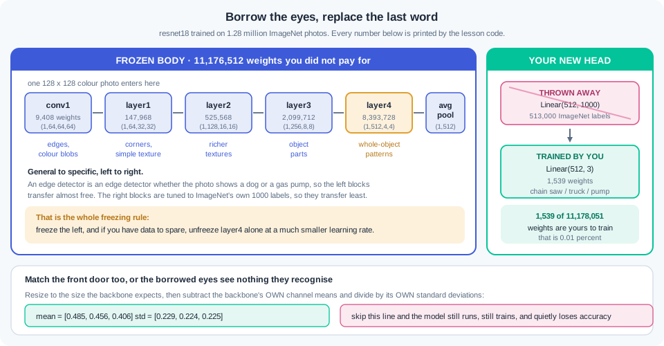
Transfer learning — taking a model trained on one large task and reusing it on your smaller one — is the highest-value trick in applied vision. The model you reuse is called a pretrained backbone, which is the body of a trained network with its final classifier removed. You keep the body and attach a new head of your own. The download for resnet18 is 44.7 MB, and it took 6 seconds on this course's connection.
Why should another team's weights help you at all? Because 2.5 showed what the layers actually learn. Early layers find edges and colour blobs, middle layers find textures, and later layers find object parts. None of that is specific to a chain saw or a gas pump, and an edge is an edge in every photograph on earth. Only the last layer names ImageNet's own 1000 classes, so only the last layer has to go.
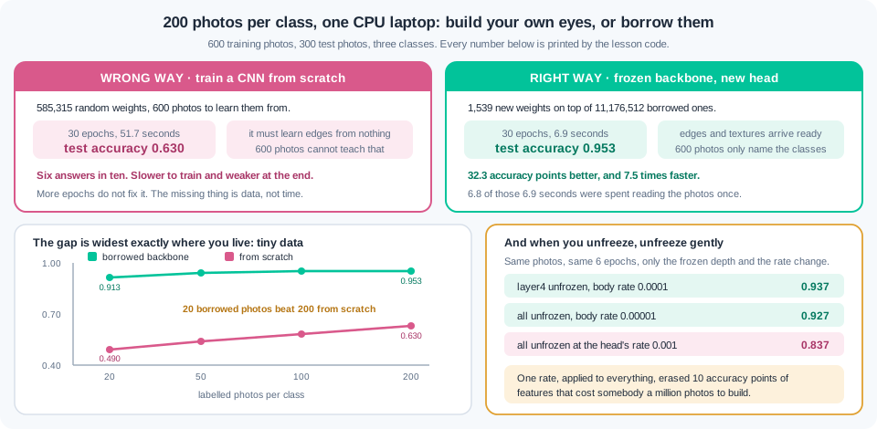
There is a wrong way and a right way to spend an evening on 600 photos. The wrong way trains 585,315 random weights from scratch and reaches 0.630 on the test set after 49.5 seconds. The right way freezes the borrowed body, trains 1,539 new weights, and reaches 0.953 in 6.3 seconds. That is 32.3 accuracy points better and about eight times faster, on the same photos and the same laptop. Amrita's six-in-ten model was not a bad model; it was a model asked to learn vision from 600 pictures.
There are two ways to use a backbone, and you will measure both. Feature extraction — freezing every borrowed weight and training only a new head — treats the backbone as a fixed camera that turns any photo into 512 numbers. Fine-tuning — letting some borrowed weights keep learning on your data — lets the backbone adjust its own idea of what matters. Extraction is faster, safer on tiny data, and often enough. Fine-tuning costs more time and can win when your images look unlike ImageNet photos.
Freezing — setting requires_grad = False so a weight receives no gradient and never moves — is one line per parameter. The order matters more than the line. Load the backbone, freeze the body, replace the head, and only then build the optimizer. Build the optimizer first and it holds a head that no longer exists, so the loss sits near 1.32 for six epochs and the model scores 0.230. That is WR-135, and the counted proof takes two prints.
When you do unfreeze, unfreeze gently. Your new head starts random, so its gradients are large and badly aimed, and at the head's own rate one epoch of those gradients flows back and damages weights that cost somebody a million photos. A differential learning rate — a different step size for each group of weights — is the fix, and PyTorch takes it as a list of parameter groups. Below, unfreezing the last block at 0.0001 scores 0.937 while unfreezing everything at 0.001 scores 0.837. Ten accuracy points is what one careless rate costs.
The input pipeline is the quietest trap in this module. A pretrained backbone was trained on inputs with ImageNet's channel means subtracted and its channel spreads divided out, so it expects that same shape of number. Feed it raw 0-to-1 pixels and nothing errors, nothing warns, and accuracy slides from 0.953 to 0.900. Feed it 0-to-255 pixels and it falls to 0.657. Ask the weights for their own transform rather than typing the numbers, because that habit survives the day you change backbones (WR-133).
How much data do you actually need? Below you measure it on the same task at 20, 50, 100 and 200 photos per class. The frozen backbone reads 0.913 with 20 photos per class, which is already better than the scratch model with ten times more. The scratch model climbs slowly from 0.490 to 0.630 and is still climbing. The rule to carry away is plain: the less data you have, the more transfer learning wins.
Check the licence before you ship, because this is a professional habit rather than a formality. Torchvision's weight objects carry their own record: the file, its size, the training recipe, and the reported ImageNet accuracy. Print it, save it beside your checkpoint, and you can answer "where did this model come from" in a client review. Some popular weights on the internet carry research-only or non-commercial terms, and finding that out after launch is an expensive way to learn.
Be honest about where this stops working. ImageNet is a set of ordinary colour photographs, so backbones trained on it transfer well to other ordinary photographs. Medical scans, satellite tiles, radar returns, and microscope slides look nothing like a holiday picture, and the borrowed features carry much less. In the far-domain check below, grey 28-pixel clothing thumbnails give the frozen backbone only 2.7 points over training from scratch, against 32.3 points on the depot photos. Transfer learning is the first thing to try, not the answer to everything.
Work inside ai-lab with torch, torchvision and pillow. One-time setup: pip install torch==2.9.* torchvision==0.24.* — the 2.3 pin plus its matching torchvision — then the resnet18 weights download once, 44.7 MB, in about 6 seconds. The photo set is Imagenette, a 98 MB folder of ordinary photographs at 160 pixels, downloaded once from https://s3.amazonaws.com/fast-ai-imageclas/imagenette2-160.tgz and unpacked into ./data. On a slow hostel connection, do the download step on Kaggle instead and copy the three class folders across; this course's rule is Kaggle first for anything heavy, and checkpoint everything. Timings below come from a plain CPU laptop with four threads.
Step 1 — open the box before you use it. What you are borrowing, block by block, with the head you must replace and the provenance you must record:
import torch, torch.nn as nn
from torchvision.models import (resnet18, ResNet18_Weights,
                                mobilenet_v3_small, MobileNet_V3_Small_Weights)

torch.set_num_threads(4)
weights = ResNet18_Weights.IMAGENET1K_V1          # a named, versioned weight set
backbone = resnet18(weights=weights)
backbone.eval()

total = sum(p.numel() for p in backbone.parameters())
print(f"resnet18, ImageNet weights: {total:,} parameters")
print(f"weights file: {weights.url.split('/')[-1]}  "
      f"{weights.meta['_file_size']:.1f} MB")
print(f"trained on : {len(weights.meta['categories'])} ImageNet classes, "
      f"top-1 {weights.meta['_metrics']['ImageNet-1K']['acc@1']}%")
print(f"recipe     : {weights.meta['recipe']}")

x = torch.zeros(1, 3, 128, 128)
print(f"\n{'block':<10s} {'output (N,C,H,W)':<22s} {'params':>12s}  what it learned")
notes = {"conv1": "edges, colour blobs", "bn1": "-", "relu": "-", "maxpool": "-",
         "layer1": "corners, simple textures", "layer2": "richer textures",
         "layer3": "object parts", "layer4": "whole-object patterns",
         "avgpool": "one number per channel", "fc": "ImageNet's 1000 labels"}
for name, mod in backbone.named_children():
    if name == "fc":
        x = torch.flatten(x, 1)
    with torch.no_grad():
        x = mod(x)
    p = sum(q.numel() for q in mod.parameters())
    print(f"{name:<10s} {str(tuple(x.shape)):<22s} {p:12,d}  {notes[name]}")

print(f"\nthe head that must go: {backbone.fc}")
print(f"  in_features  {backbone.fc.in_features}   <- the feature size you keep")
print(f"  out_features {backbone.fc.out_features}   <- ImageNet labels you do not want")
head_p = sum(q.numel() for q in backbone.fc.parameters())
print(f"  body {total - head_p:,} params kept, head {head_p:,} params thrown away")
print(f"\nthe backbone's own documented transform:\n{weights.transforms()}")

mw = MobileNet_V3_Small_Weights.IMAGENET1K_V1
mobilenet_v3_small(weights=mw)
print(f"\n{'model':<20s} {'params':>12s} {'weights MB':>11s} {'GFLOPs':>8s} {'top-1':>7s}")
for label, w in (("resnet18", weights), ("mobilenet_v3_small", mw)):
    print(f"{label:<20s} {w.meta['num_params']:12,d} {w.meta['_file_size']:11.1f}"
          f" {w.meta['_ops']:8.3f} {w.meta['_metrics']['ImageNet-1K']['acc@1']:7.2f}")
Output:
resnet18, ImageNet weights: 11,689,512 parameters
weights file: resnet18-f37072fd.pth  44.7 MB
trained on : 1000 ImageNet classes, top-1 69.758%
recipe     : https://github.com/pytorch/vision/tree/main/references/classification#resnet

block      output (N,C,H,W)             params  what it learned
conv1      (1, 64, 64, 64)               9,408  edges, colour blobs
bn1        (1, 64, 64, 64)                 128  -
relu       (1, 64, 64, 64)                   0  -
maxpool    (1, 64, 32, 32)                   0  -
layer1     (1, 64, 32, 32)             147,968  corners, simple textures
layer2     (1, 128, 16, 16)            525,568  richer textures
layer3     (1, 256, 8, 8)            2,099,712  object parts
layer4     (1, 512, 4, 4)            8,393,728  whole-object patterns
avgpool    (1, 512, 1, 1)                    0  one number per channel
fc         (1, 1000)                   513,000  ImageNet's 1000 labels

the head that must go: Linear(in_features=512, out_features=1000, bias=True)
  in_features  512   <- the feature size you keep
  out_features 1000   <- ImageNet labels you do not want
  body 11,176,512 params kept, head 513,000 params thrown away

the backbone's own documented transform:
ImageClassification(
    crop_size=[224]
    resize_size=[256]
    mean=[0.485, 0.456, 0.406]
    std=[0.229, 0.224, 0.225]
    interpolation=InterpolationMode.BILINEAR
)

model                      params  weights MB   GFLOPs   top-1
resnet18               11,689,512        44.7    1.814   69.76
mobilenet_v3_small      2,542,856         9.8    0.057   67.67
Five readings, in the order you will use them. First the shape trace: a 128-pixel photo shrinks 64, 32, 16, 8, 4 through the blocks and leaves avgpool as 512 numbers, so 512 is the number your new head must accept. Second the parameter column: layer4 alone holds 8,393,728 weights, three quarters of the whole body, which is why unfreezing it costs real time. Third the head: in_features=512, out_features=1000, and you read those from the object rather than typing them, because mobilenet_v3_small would give you 576 instead. Fourth the transform block, which is the module's most important printout — resize 256, crop 224, and those six normalisation numbers are part of the weights, not part of your taste. Fifth the provenance line: a file name, a size, a recipe URL and 69.758% top-1 accuracy is what you paste into a client document when somebody asks where the model came from, and the mobilenet row shows the cheaper option at 0.057 GFLOPs against 1.814, which matters the day this runs on a phone.
Step 2 — the small photo set, and a front door the backbone recognises. Save this as depot.py; every later step imports it:
import os, time, copy, torch, torch.nn as nn
from PIL import Image
from torch.utils.data import DataLoader, TensorDataset
from torchvision import transforms
from torchvision.models import resnet18, ResNet18_Weights

torch.set_num_threads(4)
ROOT = "./data/imagenette2-160"
WNID = {"n03000684": "chain saw", "n03417042": "garbage truck",
        "n03425413": "gas pump"}
NAMES = [WNID[w] for w in sorted(WNID)]
MEAN = torch.tensor([0.485, 0.456, 0.406]).view(1, 3, 1, 1)   # from the weights
STD = torch.tensor([0.229, 0.224, 0.225]).view(1, 3, 1, 1)
loss_fn = nn.CrossEntropyLoss()

read = transforms.Compose([transforms.Resize(144), transforms.CenterCrop(128),
                           transforms.ToTensor()])

def load(split, per_class, skip=0):
    xs, ys = [], []
    for ci, w in enumerate(sorted(WNID)):
        folder = os.path.join(ROOT, split, w)
        for fn in sorted(os.listdir(folder))[skip:skip + per_class]:
            xs.append(read(Image.open(os.path.join(folder, fn)).convert("RGB")))
            ys.append(ci)
    return torch.stack(xs), torch.tensor(ys)

Xtr_raw, ytr = load("train", 200)            # 200 photos per class
Xva_raw, yva = load("train", 60, skip=200)   # 60 more, never trained on
Xte_raw, yte = load("val", 100)              # 100 held back for the final score

def norm(x, mean=MEAN, std=STD):
    return (x - mean) / std

def scratch_cnn():                           # 2.5's CNN, widened for 128 px colour
    return nn.Sequential(
        nn.Conv2d(3, 16, 3, padding=1), nn.ReLU(), nn.MaxPool2d(2),
        nn.Conv2d(16, 32, 3, padding=1), nn.ReLU(), nn.MaxPool2d(2),
        nn.Conv2d(32, 64, 3, padding=1), nn.ReLU(), nn.MaxPool2d(2),
        nn.Conv2d(64, 64, 3, padding=1), nn.ReLU(), nn.MaxPool2d(2),
        nn.Flatten(), nn.Linear(64 * 8 * 8, 128), nn.ReLU(), nn.Linear(128, 3))

@torch.no_grad()
def accuracy(net, X, y, bs=64):
    net.eval()
    return sum(int((net(X[i:i+bs]).argmax(1) == y[i:i+bs]).sum())
               for i in range(0, len(X), bs)) / len(X)

@torch.no_grad()
def features(body, X, bs=32):        # run the frozen body once, keep the 512 numbers
    body.eval()
    return torch.cat([body(X[i:i+bs]).flatten(1) for i in range(0, len(X), bs)])

def train(net, X, y, Xv, yv, epochs, opt, bs=32, seed=7, log=None):
    dl = DataLoader(TensorDataset(X, y), batch_size=bs, shuffle=True,
                    generator=torch.Generator().manual_seed(seed))
    best, state = -1.0, None
    for ep in range(1, epochs + 1):
        net.train()
        total = 0.0
        for xb, yb in dl:
            opt.zero_grad()
            l = loss_fn(net(xb), yb)
            l.backward(); opt.step()
            total += l.item() * len(xb)
        va = accuracy(net, Xv, yv)
        if va > best:
            best, state = va, copy.deepcopy(net.state_dict())   # 2.4's rewind
        if log is not None:
            log.append((ep, total / len(X), va))
    net.load_state_dict(state)
    return best

if __name__ == "__main__":
    print(f"{'split':<8s} {'shape (N,C,H,W)':<22s} {'per class':>10s}")
    for lbl, X in (("train", Xtr_raw), ("val", Xva_raw), ("test", Xte_raw)):
        print(f"{lbl:<8s} {str(tuple(X.shape)):<22s} {len(X)//3:10d}")
    print("classes:", NAMES)

    Xn = norm(Xtr_raw)
    print(f"\n{'pipeline':<26s} {'min':>8s} {'max':>8s} {'mean':>8s} {'std':>8s}")
    print(f"{'ToTensor only (0-1)':<26s} {Xtr_raw.min():8.3f} {Xtr_raw.max():8.3f}"
          f" {Xtr_raw.mean():8.3f} {Xtr_raw.std():8.3f}")
    print(f"{'+ ImageNet mean/std':<26s} {Xn.min():8.3f} {Xn.max():8.3f}"
          f" {Xn.mean():8.3f} {Xn.std():8.3f}")
    print("per-channel mean after normalisation:",
          [round(float(Xn[:, c].mean()), 3) for c in range(3)])

    body = resnet18(weights=ResNet18_Weights.IMAGENET1K_V1)
    body.fc = nn.Identity()
    print()
    for size in (128, 224):
        x = torch.nn.functional.interpolate(Xte_raw[:60], size=size,
                                            mode="bilinear", antialias=True)
        t0 = time.perf_counter(); features(body, norm(x))
        dt = time.perf_counter() - t0
        print(f"features for 60 photos at {size:3d} px: {dt:4.1f} s"
              f" ({dt/60*1000:5.0f} ms each)")
Output:
split    shape (N,C,H,W)         per class
train    (600, 3, 128, 128)            200
val      (180, 3, 128, 128)             60
test     (300, 3, 128, 128)            100
classes: ['chain saw', 'garbage truck', 'gas pump']

pipeline                        min      max     mean      std
ToTensor only (0-1)           0.000    1.000    0.454    0.277
+ ImageNet mean/std          -2.118    2.640    0.021    1.227
per-channel mean after normalisation: [-0.057, 0.009, 0.112]

features for 60 photos at 128 px:  0.3 s (    6 ms each)
features for 60 photos at 224 px:  0.9 s (   14 ms each)
Read the two pipeline rows together, because that pair is the whole point of the step. ToTensor leaves pixels between 0.000 and 1.000 with a mean of 0.454 and a spread of 0.277, which is what 2.5's from-scratch CNN was happy with. After the backbone's own mean and spread are applied, the numbers run from -2.118 to 2.640 with a mean of 0.021 and a spread of 1.227, centred near zero and spread near one, which is what every filter inside resnet18 was trained to see. The three per-channel means, -0.057, 0.009 and 0.112, are close to zero but not equal to it, and that is correct: depot photos are not ImageNet, so the subtraction lands near zero rather than on it. The last two lines are the CPU compromise this course makes on purpose. The documented crop is 224 pixels and costs 14 ms per photo, while 128 pixels costs 6 ms, so the whole 1,080-photo set takes about 6 seconds instead of 15. Change the resize and the crop when compute forces you; never change the mean and the spread, because those belong to the weights.
Step 3 — the bake-off: scratch against frozen against fine-tuned. Same 600 photos, same 300 test photos, one honest clock:
import time, torch, torch.nn as nn
from torchvision.models import resnet18, ResNet18_Weights
from depot import *

Xtr, Xva, Xte = norm(Xtr_raw), norm(Xva_raw), norm(Xte_raw)
W = ResNet18_Weights.IMAGENET1K_V1
print(f"{'approach':<26s} {'trainable':>11s} {'ep':>4s} {'sec':>6s}"
      f" {'val':>7s} {'test':>7s}")

# ---- A. from scratch: no borrowed weights at all -------------------------
torch.manual_seed(7)
net = scratch_cnn()
opt = torch.optim.Adam(net.parameters(), lr=1e-3)
t0 = time.perf_counter()
va = train(net, Xtr, ytr, Xva, yva, 30, opt)
print(f"{'A from scratch':<26s} {sum(p.numel() for p in net.parameters()):11,d}"
      f" {30:4d} {time.perf_counter()-t0:6.1f} {va:7.3f}"
      f" {accuracy(net, Xte, yte):7.3f}")

# ---- B. feature extraction: freeze the body, train a new head ------------
torch.manual_seed(7)
body = resnet18(weights=W)
body.fc = nn.Identity()                      # drop ImageNet's 1000-way head
for p in body.parameters():
    p.requires_grad = False                  # freeze every borrowed weight
t0 = time.perf_counter()
Ftr, Fva, Fte = features(body, Xtr), features(body, Xva), features(body, Xte)
extract = time.perf_counter() - t0
torch.manual_seed(7)
head = nn.Linear(512, 3)
opt = torch.optim.Adam(head.parameters(), lr=1e-3)
va = train(head, Ftr, ytr, Fva, yva, 30, opt)
print(f"{'B frozen features':<26s} {sum(p.numel() for p in head.parameters()):11,d}"
      f" {30:4d} {time.perf_counter()-t0:6.1f} {va:7.3f}"
      f" {accuracy(head, Fte, yte):7.3f}   (extract {extract:.1f}s of it)")

# ---- C. fine-tune the last block, gently --------------------------------
torch.manual_seed(7)
ft = resnet18(weights=W)
ft.fc = nn.Linear(ft.fc.in_features, 3)      # read in_features, never type it
for p in ft.parameters():
    p.requires_grad = False
for p in ft.layer4.parameters():
    p.requires_grad = True
for p in ft.fc.parameters():
    p.requires_grad = True
opt = torch.optim.Adam([{"params": ft.layer4.parameters(), "lr": 1e-4},
                        {"params": ft.fc.parameters(), "lr": 1e-3}])
t0 = time.perf_counter()
va = train(ft, Xtr, ytr, Xva, yva, 6, opt)
live = sum(p.numel() for p in ft.parameters() if p.requires_grad)
print(f"{'C fine-tune layer4':<26s} {live:11,d} {6:4d}"
      f" {time.perf_counter()-t0:6.1f} {va:7.3f} {accuracy(ft, Xte, yte):7.3f}")

with torch.no_grad():
    pred = head(Fte).argmax(1)
print(f"\nB's mistakes, 100 test photos per class (rows true, columns predicted):")
print(f"{'':<15s}" + "".join(f"{n:>15s}" for n in NAMES))
for c in range(3):
    row = [int(((yte == c) & (pred == p)).sum()) for p in range(3)]
    print(f"{NAMES[c]:<15s}" + "".join(f"{v:15d}" for v in row))
Output:
approach                     trainable   ep    sec     val    test
A from scratch                 585,315   30   49.5   0.617   0.630
B frozen features                1,539   30    6.3   0.961   0.953   (extract 6.2s of it)
C fine-tune layer4           8,395,267    6   36.2   0.961   0.937

B's mistakes, 100 test photos per class (rows true, columns predicted):
                     chain saw  garbage truck       gas pump
chain saw                   96              3              1
garbage truck                3             94              3
gas pump                     3              1             96
Four readings, and the fourth is the one most courses skip. First, the size of the win: 0.953 against 0.630 is 32.3 accuracy points from the same 600 photos, and it took 6.3 seconds against 49.5. Second, where those 6.3 seconds went — 6.2 of them were the single pass that turned 1,080 photos into 512 numbers each, so the actual training of 1,539 weights took about a tenth of a second, and rerunning the head with different settings is now instant. Third, the trainable column tells you why row A had no chance: 585,315 random weights, 600 photos, and the model must discover edge detectors before it can start on chain saws. Fourth, and this is the honest part, fine-tuning did not win. Row C unfroze 8,395,267 weights, took six times longer than row B, and landed at 0.937 rather than 0.953, because depot photos already look like ImageNet photos and 600 of them are too few to improve an 8-million-weight block. Keep the frozen score as the number a fine-tune has to beat, and be willing to report that it did not. The confusion table shows the remaining 14 mistakes spread evenly, 96, 94 and 96 correct per class, with no pair collapsing into another — there is no single weak class to attack here.
Step 4 — the front door, five ways. Same frozen backbone, same head, only the pipeline changes:
import torch, torch.nn as nn
from torchvision.models import resnet18, ResNet18_Weights
from depot import *

body = resnet18(weights=ResNet18_Weights.IMAGENET1K_V1)
body.fc = nn.Identity()
for p in body.parameters():
    p.requires_grad = False
HALF = torch.tensor([0.5, 0.5, 0.5]).view(1, 3, 1, 1)

def bake(label, pipeline):
    torch.manual_seed(7)
    F = [features(body, pipeline(X)) for X in (Xtr_raw, Xva_raw, Xte_raw)]
    head = nn.Linear(512, 3)
    opt = torch.optim.Adam(head.parameters(), lr=1e-3)
    train(head, F[0], ytr, F[1], yva, 30, opt)
    x = pipeline(Xte_raw)
    print(f"{label:<40s} {float(x.mean()):+8.3f} {float(x.std()):7.3f}"
          f" {accuracy(head, F[2], yte):9.3f}")

print(f"{'input pipeline':<40s} {'mean':>8s} {'std':>7s} {'test acc':>9s}")
bake("ImageNet mean/std, the documented one", lambda x: norm(x))
bake("no Normalize at all, raw 0-1 pixels", lambda x: x)
bake("wrong stats: mean 0.5, std 0.5", lambda x: norm(x, HALF, HALF))
bake("BGR channel order, right stats", lambda x: norm(x)[:, [2, 1, 0]])
bake("0-255 pixels, ToTensor scale undone", lambda x: x * 255.0)
Output:
input pipeline                               mean     std  test acc
ImageNet mean/std, the documented one      -0.019   1.196     0.953
no Normalize at all, raw 0-1 pixels        +0.445   0.271     0.900
wrong stats: mean 0.5, std 0.5             -0.111   0.541     0.940
BGR channel order, right stats             -0.019   1.196     0.927
0-255 pixels, ToTensor scale undone      +113.399  69.002     0.657
Every row ran without an error, a warning or a crash, and that is the lesson. The damage tracks the size of the mismatch. Dropping Normalize entirely leaves the mean at 0.445 instead of near zero and costs 5.3 points, which on a busy day looks like ordinary variance and gets blamed on the dataset. Using mean 0.5 and spread 0.5 is closer to right and costs 1.3 points, small enough to hide forever. Swapping red and blue costs 2.6 points while leaving the mean and spread columns identical to the correct row, so those two prints alone cannot catch it — only reading the pipeline can. Leaving pixels on the 0-to-255 scale pushes the mean to 113.399 and the spread to 69.002, saturates the early layers, and costs 29.6 points. Two habits close all five holes: take the numbers from weights.transforms() instead of typing them, and assert once per run that a training batch has a mean inside plus or minus 0.5 and a spread between 0.5 and 2.0 (WR-133).
Step 5 — freezing, counted rather than assumed. Five configurations, an audit before any training, and three epochs of consequences:
import time, torch, torch.nn as nn
from torchvision.models import resnet18, ResNet18_Weights
from depot import *

Xtr, Xva, Xte = norm(Xtr_raw), norm(Xva_raw), norm(Xte_raw)

def fresh(freeze_body=True):
    torch.manual_seed(7)
    m = resnet18(weights=ResNet18_Weights.IMAGENET1K_V1)
    if freeze_body:
        for p in m.parameters():
            p.requires_grad = False
    return m

cases = []
m = fresh(); m.fc = nn.Linear(512, 3)
for p in m.fc.parameters():
    p.requires_grad = False                        # bug 1: the head froze too
cases.append(("1 head frozen with the body", m,
              torch.optim.Adam(m.parameters(), lr=1e-3)))

m = fresh()
o = torch.optim.Adam(m.fc.parameters(), lr=1e-3)   # bug 2: optimizer built first
m.fc = nn.Linear(512, 3)                           # the head it holds no longer exists
cases.append(("2 optimizer built before head", m, o))

m = fresh(); m.fc = nn.Linear(512, 3)              # right: freeze, replace, optimise
cases.append(("3 freeze, replace, optimise head", m,
              torch.optim.Adam(m.fc.parameters(), lr=1e-3)))

m = fresh(freeze_body=False); m.fc = nn.Linear(512, 3)
cases.append(("4 nothing frozen, one lr 1e-3", m,
              torch.optim.Adam(m.parameters(), lr=1e-3)))

m = fresh(freeze_body=False); m.fc = nn.Linear(512, 3)
cases.append(("5 all live, body 1e-5 head 1e-3", m, torch.optim.Adam(
    [{"params": [p for n, p in m.named_parameters() if not n.startswith("fc")],
      "lr": 1e-5},
     {"params": m.fc.parameters(), "lr": 1e-3}])))

print(f"{'configuration':<32s} {'trainable':>11s} {'frozen':>11s}"
      f" {'in optimizer':>12s} {'of it live':>11s}")
for label, m, o in cases:
    live = sum(p.numel() for p in m.parameters() if p.requires_grad)
    dead = sum(p.numel() for p in m.parameters() if not p.requires_grad)
    held = sum(p.numel() for g in o.param_groups for p in g["params"])
    held_live = sum(p.numel() for g in o.param_groups
                    for p in g["params"] if p.requires_grad)
    print(f"{label:<32s} {live:11,d} {dead:11,d} {held:12,d} {held_live:11,d}")

print(f"\n{'configuration':<32s} {'ep1 loss':>9s} {'ep6 loss':>9s} {'sec':>6s}"
      f" {'test acc':>9s}")
for label, m, o in cases:
    log, t0 = [], time.perf_counter()
    try:
        train(m, Xtr, ytr, Xva, yva, 6, o, log=log)
    except RuntimeError as e:
        print(f"{label:<32s}  RuntimeError: {str(e)[:44]}")
        continue
    print(f"{label:<32s} {log[0][1]:9.4f} {log[-1][1]:9.4f}"
          f" {time.perf_counter()-t0:6.1f} {accuracy(m, Xte, yte):9.3f}")
Output:
configuration                      trainable      frozen in optimizer  of it live
1 head frozen with the body                0  11,178,051   11,178,051           0
2 optimizer built before head          1,539  11,176,512      513,000           0
3 freeze, replace, optimise head       1,539  11,176,512        1,539       1,539
4 nothing frozen, one lr 1e-3     11,178,051           0   11,178,051  11,178,051
5 all live, body 1e-5 head 1e-3   11,178,051           0   11,178,051  11,178,051

configuration                     ep1 loss  ep6 loss    sec  test acc
1 head frozen with the body       RuntimeError: element 0 of tensors does not require grad a
2 optimizer built before head       1.3237    1.3161   31.4     0.230
3 freeze, replace, optimise head    0.9369    0.2340   32.0     0.887
4 nothing frozen, one lr 1e-3       0.6473    0.0726   61.6     0.837
5 all live, body 1e-5 head 1e-3     0.8227    0.0581   63.2     0.927
Read the audit table first, because it predicts every row of the second table before a single epoch runs. Row 1 has 0 trainable weights, so backward() refuses to run and you get a loud error in the first second — annoying, and the kindest failure on this page. Row 2 is the dangerous one: 1,539 trainable weights and 513,000 weights held by the optimizer, of which 0 are live, which means the optimizer is faithfully updating a head that was thrown away. Nothing errors, the loss reads 1.3237 and then 1.3161, and the model scores 0.230 on three classes, below the 0.333 a coin would give. That is WR-135, and the two counts on row 3 — 1,539 trainable, 1,539 held, all live — are the shape a healthy setup has. Now the last two rows, which are WR-134. Both unfroze all 11,178,051 weights, both took about a minute, and both show a training loss falling faster than row 3. Row 4 used one rate of 0.001 for everything and scored 0.837; row 5 gave the borrowed weights 0.00001 and the new head 0.001 and scored 0.927. The training loss was the trap: row 4 ended at 0.0726, the lowest on the table, while its test score was 9 points below row 5. That is 2.4's lesson again — the training column is not the score.
Step 6 — how much data, and where the borrowed eyes stop helping. The curve first, then a domain ImageNet never saw:
import torch, torch.nn as nn
from torchvision import datasets, transforms
from torchvision.models import resnet18, ResNet18_Weights
from depot import *

Xtr, Xva, Xte = norm(Xtr_raw), norm(Xva_raw), norm(Xte_raw)
body = resnet18(weights=ResNet18_Weights.IMAGENET1K_V1)
body.fc = nn.Identity()
for p in body.parameters():
    p.requires_grad = False
Ftr, Fva, Fte = features(body, Xtr), features(body, Xva), features(body, Xte)

def first_n_per_class(y, n):
    return torch.cat([torch.nonzero(y == c).flatten()[:n] for c in range(3)])

def scratch_score(X, y, Xv, yv, Xt, yt):
    torch.manual_seed(7)
    net = scratch_cnn()
    train(net, X, y, Xv, yv, 30, torch.optim.Adam(net.parameters(), lr=1e-3))
    return accuracy(net, Xt, yt)

def frozen_score(F, y, Fv, yv, Ft, yt, dim=512):
    torch.manual_seed(7)
    head = nn.Linear(dim, 3)
    train(head, F, y, Fv, yv, 30, torch.optim.Adam(head.parameters(), lr=1e-3))
    return accuracy(head, Ft, yt)

print(f"{'photos per class':>16s} {'total':>6s} {'scratch':>8s} {'frozen':>7s} {'gap':>7s}")
for n in (20, 50, 100, 200):
    i = first_n_per_class(ytr, n)
    a = scratch_score(Xtr[i], ytr[i], Xva, yva, Xte, yte)
    b = frozen_score(Ftr[i], ytr[i], Fva, yva, Fte, yte)
    print(f"{n:16d} {n*3:6d} {a:8.3f} {b:7.3f} {b-a:+7.3f}")

# ---- a domain the backbone never saw: grey 28-pixel clothing thumbnails ----
tt = transforms.ToTensor()
fm_tr = datasets.FashionMNIST("./data", train=True, download=True, transform=tt)
fm_te = datasets.FashionMNIST("./data", train=False, download=True, transform=tt)
g = torch.Generator().manual_seed(42)
KEEP = [2, 4, 6]                                   # pullover, coat, shirt

def grab(ds, per):
    xs, ys, seen = [], [], {c: 0 for c in KEEP}
    for i in torch.randperm(len(ds), generator=g).tolist():
        x, y = ds[i]
        if y in KEEP and seen[y] < per:
            seen[y] += 1; xs.append(x); ys.append(KEEP.index(y))
        if all(v == per for v in seen.values()):
            break
    X = torch.nn.functional.interpolate(torch.stack(xs).repeat(1, 3, 1, 1),
                                        size=128, mode="bilinear", antialias=True)
    return norm(X), torch.tensor(ys)

Gtr, gtr = grab(fm_tr, 200); Gva, gva = grab(fm_tr, 60); Gte, gte = grab(fm_te, 100)
print("\nfar from ImageNet: FashionMNIST pullover / coat / shirt, grey, 28 px")
print(f"{'approach':<26s} {'test acc':>9s}")
print(f"{'from scratch':<26s} {scratch_score(Gtr, gtr, Gva, gva, Gte, gte):9.3f}")
print(f"{'frozen ImageNet features':<26s} "
      f"{frozen_score(features(body, Gtr), gtr, features(body, Gva), gva, features(body, Gte), gte):9.3f}")
Output:
photos per class  total  scratch  frozen     gap
              20     60    0.490   0.913  +0.423
              50    150    0.540   0.943  +0.403
             100    300    0.580   0.953  +0.373
             200    600    0.630   0.953  +0.323

far from ImageNet: FashionMNIST pullover / coat / shirt, grey, 28 px
approach                    test acc
from scratch                   0.743
frozen ImageNet features       0.770
Read the curve from the top, because the top row is the one that changes how you plan a project. With 20 photos per class — 60 photos in total, an afternoon of labelling — the frozen backbone scores 0.913, which beats the from-scratch model trained on ten times more data by 28 points. The gap narrows as data grows, 0.423 to 0.403 to 0.373 to 0.323, and it would keep narrowing: with tens of thousands of images per class, training from scratch becomes competitive again. Notice also that the frozen column stops moving after 100 photos per class, at 0.953, while the scratch column is still climbing at 200. That flat top is telling you where your next hour belongs, and it is not on more photos of the same three machines. Then the far-domain block, which is the honesty check. Grey 28-pixel clothing thumbnails are nothing like ImageNet's colour photographs, and there the borrowed features buy 2.7 points, 0.770 against 0.743, instead of 32.3. Medical scans, satellite tiles and radar returns sit in that second world, and on those a smaller network trained from scratch or a backbone pretrained on similar images is often the better call.
Work inside ai-lab with torch, torchvision and pillow, and keep depot.py from Step 2 in the folder, because every exercise imports it. Everything is seeded, so where a loss or an accuracy is given your output should land within about 1% of it — seeded torch runs vary slightly across builds — while shapes and counts should match exactly; wall-clock seconds will differ with your machine and that is expected. If a fine-tuning run is too slow on your laptop, move that one part to a Kaggle CPU notebook and save the checkpoint, which is this course's standing rule.
If your numbers are close but not identical, triage in a fixed order before touching your code. Everything off by a little — every value drifting in the last decimal or two — points at a library version: run pip show torch, compare it with the pinned install line, and match the pin, because the printed numbers were produced on that version. One number wildly off while the rest agree points at stale state: restart from a fresh kernel or a fresh python and run the file top to bottom, since seeded draws only reproduce when they happen in the same order from a clean start. Only when both checks pass and the numbers still disagree should you suspect your own logic — diff your script line by line against the printed code.
Read the backbone before you use it. Create inspect_backbone.py. Part one: load resnet18 with ResNet18_Weights.IMAGENET1K_V1 and print its total parameter count, its per-block parameter counts, and the output shape after every block for a (1, 3, 128, 128) input. Part two: print the head's in_features and out_features, then do the same for mobilenet_v3_small and for resnet34, building a three-row table of model name, parameter count, weights file size in MB, GFLOPs, ImageNet top-1 accuracy, and feature width — the number your new head must accept. Part three: the provenance record. For each of the three, print the weights file name, the recipe URL, and the number of ImageNet classes, then write those three rows into a MODEL_CARD.md with one sentence saying which model you would ship on an 8GB laptop and why. Part four: print weights.transforms() for all three and write one comment naming what is identical across them and what is not. Check: resnet18 prints 11,689,512 parameters with a 44.7 MB file and a head of in_features=512, out_features=1000; layer4 alone holds 8,393,728 parameters, which is over 70 percent of the body; mobilenet_v3_small prints 2,542,856 parameters, 9.8 MB, 0.057 GFLOPs against resnet18's 1.814, and a feature width of 576, not 512; resnet34 prints roughly 21.8 million parameters; all three transforms print the same mean=[0.485, 0.456, 0.406] and std=[0.229, 0.224, 0.225], and your comment says the normalisation is shared because all three were trained on the same ImageNet pixels; and MODEL_CARD.md names a file, a size and a recipe URL for each row.
The bake-off, then the data curve. Create bakeoff.py and import depot.py. Part one: reproduce Step 3's three rows exactly — from scratch, frozen features, and layer4 fine-tuned — printing trainable parameters, epochs, wall-clock seconds, best validation accuracy and test accuracy for each. Part two: break the frozen run's time into two numbers, the one-pass feature extraction and the head training, then retrain the head three more times at learning rates 0.01, 0.003 and 0.0003 on the already-extracted features and report the seconds each retrain took. Part three: reproduce the data curve at 20, 50, 100 and 200 photos per class for both the scratch model and the frozen head, printing the gap column. Part four: print the confusion table for your best model and write three comment sentences — which approach you would ship, what the flat top of the frozen column means for your next hour of work, and what the curve says about a teammate who wants to label another 200 photos per class. Check: your from-scratch row reads test 0.630 in about 50 seconds with 585,315 parameters; frozen features reads 0.953 in about 6 seconds with 1,539 trainable parameters, and at least 90 percent of that time is the single extraction pass, so each head retrain finishes in well under a second; fine-tuning layer4 reads 0.937 with 8,395,267 trainable parameters and takes about six times longer than the frozen run, and your comment states plainly that it lost to the frozen baseline; the curve reads 0.490 / 0.913, 0.540 / 0.943, 0.580 / 0.953 and 0.630 / 0.953; and your confusion table shows 96, 94 and 96 correct per class with no pair of classes collapsing into one.
The freeze-depth lab. Create freeze_lab.py. Part one, the audit function: write report(model, opt) that prints four numbers — trainable parameters, frozen parameters, parameters held by the optimizer, and how many of those held parameters are live — and refuses to continue when the last number is zero. Part two, the sweep: run six configurations for six epochs each on the same 600 photos, printing for every one the four audit numbers, epoch-1 and epoch-6 training loss, wall-clock seconds, training accuracy, validation accuracy and test accuracy. The six are: everything frozen except the head; layer4 plus head at body rate 0.0001; layer3 and layer4 plus head at 0.0001; everything unfrozen at a single 0.001; everything unfrozen with body 0.00001 and head 0.001; and everything frozen including the head. Part three: build one table sorted by test accuracy, add a column for the training-minus-validation accuracy gap, and mark which rows overfit. Part four: pick a configuration to ship and defend it in four comment sentences that cite accuracy, seconds and the overfitting gap, then state which row you would pick instead if the client gave you 5,000 photos per class and an afternoon of GPU time. Check: the everything-frozen-including-head row raises RuntimeError: element 0 of tensors does not require grad and your audit function catches it first with a trainable count of 0 out of 11,178,051; the frozen-head row reads test 0.887 at six epochs; layer4 at 1e-4 reads 0.937; everything unfrozen at 1e-3 reads 0.837 while showing the LOWEST epoch-6 training loss on the table, near 0.0726, and your comment names that row as proof that training loss is not the score; everything unfrozen at 1e-5 reads 0.927; your table shows the unfrozen rows taking roughly twice the seconds of the frozen ones; and your defence names the frozen-feature model from exercise 2 as the baseline any fine-tune had to beat.
Bring your own three classes. Create my_classes.py and build a dataset nobody has trained on before. Part one, collect about 150 photos across three classes, 50 each, in folders named after the classes. Option A, the phone route: photograph three things around you that a model could plausibly be asked to sort — three kinds of packaged snack on a kirana shelf, three coin denominations, three types of two-wheeler — under varied light and angle, and copy them across. Option B, the offline route, if you have no camera or no time: take three classes you have not used tonight from the Imagenette folders you already downloaded, or three classes from CIFAR-10, and take only 50 training images from each. Part two: run them through Step 2's pipeline unchanged — resize, centre crop, ToTensor, and the backbone's own mean and spread — then split 50 per class into 35 train, 5 validation and 10 test, and print the three shapes plus the class counts. Part three: extract features once with the frozen resnet18 body, train a Linear(512, 3) head, and report test accuracy, the full confusion table, and the three photos your model was most confident about while being wrong. Part four: write four comment sentences — your honest accuracy, which pair of classes confused the model most, whether the confusion is a labelling problem or a genuine visual one, and how many more photos of which class you would collect next. Check: your folder layout and counts print correctly with 35, 5 and 10 photos per class, and the training tensor prints as (105, 3, 128, 128); your normalised training batch has a mean between -0.5 and +0.5 and a spread between 0.5 and 2.0, asserted in code, not eyeballed; feature extraction for all 150 photos finishes in about one second on CPU and the head trains in well under a second; your reported accuracy comes from the 30 test photos only and you state it even if it is poor, with phone-photo sets of three everyday objects usually landing between 0.70 and 0.95; your confusion table sums to 30; and your comments name a specific next action tied to a specific class rather than "collect more data".
Three transfer failures cover most of this module's pain, and two of them are silent. Each has a War Room entry with the full diagnosis path:
- WR-133 — the backbone fed the wrong pixels. A pretrained body was handed inputs it was never trained on, so every layer drifted and the score slid without a single warning: raw 0-to-1 pixels cost 5.3 accuracy points, a BGR channel swap cost 2.6, and 0-to-255 pixels cost 29.6; the fix is to take the resize, the crop, the mean and the spread from
weights.transforms()rather than typing them, and to assert the batch statistics once per run. - WR-134 — the unfreeze that erased the backbone. A working frozen model was fully unfrozen at the head's own learning rate, so the random head's first gradients overwrote features built from millions of photos: the training loss fell faster than ever while the test score dropped from 0.937 to 0.837; the fix is two stages, a frozen baseline saved first, then the last block alone at a rate ten to a hundred times smaller, with parameter groups printed before the first step.
- WR-135 — the frozen model that never learned. The optimizer was built one line before the head was replaced, so it held 513,000 weights of which none were live: the loss sat near 1.32 for six epochs and the model scored 0.230 on three classes; the fix is the fixed order — load, freeze, replace the head, then build the optimizer — plus an assertion that the trainable count is above zero and matches what the optimizer holds.
A pretrained backbone is a trained body whose early layers found edges and textures that help in any photograph, so only its final head has to go. On 600 depot photos, feature extraction with a frozen resnet18 scored 0.953 in 6.3 seconds while the same CNN trained from scratch scored 0.630 in 49.5 seconds. Fine-tuning the last block at a much smaller rate reached 0.937 and lost to the frozen baseline, while unfreezing everything at the head's own rate fell to 0.837. Match the input pipeline to the weights, count trainable parameters before you train, and read the licence and the recipe before you ship. The gap is widest where you actually live: with 20 photos per class the borrowed backbone scored 0.913 against 0.490, and it narrows on domains far from ordinary photographs.
- Document and KYC pipelines at Indian banks and fintechs classify and route scanned Aadhaar cards, PAN cards and cheques. A frozen ImageNet backbone with a small head handles the routing on a few hundred labelled scans per type, which is all a compliance team can label in a week.
- Crop and pest apps for farmers start from a pretrained backbone because a village dataset holds hundreds of leaf photos, not millions. Teams freeze the body for the first release, then fine-tune the last block once field photos accumulate over a season.
- Shelf and stock audits for kirana and retail chains classify product photos taken by field staff on cheap phones. New products arrive every month with fifty photos each, and a frozen backbone with a retrained head is the only approach that keeps up with that pace.
Answer these before opening the gate assessment. Each question names its type.
type=interpretation— A bake-off table reads: from scratch0.630in 49.5 s with 585,315 trainable weights, frozen features0.953in 6.3 s with 1,539, fine-tuned layer40.937in 36.2 s with 8,395,267. State which model you would ship and why, say what the fine-tuning row tells you about the size of this dataset, and name the one number you would report to a client who asks "how good is it".type=debug— A freeze audit printstrainable 1,539,frozen 11,176,512,in optimizer 513,000,of it live 0, and training loss reads 1.3237 then 1.3161 over six epochs. Name the exact ordering mistake in the setup code, give the corrected order in four steps, and state the two-line assertion you would add so this fails in the first second next time.type=output-prediction— A pipeline sends 0-to-1 pixels straight into a frozen resnet18 with noNormalizestep, and a second run multiplies those pixels by 255 instead. Predict the printed batch mean and spread for each run, predict which of the two loses more accuracy, and say whether either run raises an error.type=scenario-judgement— With 40 labelled X-ray images per class and no GPU, a teammate proposes downloading an ImageNet backbone and fine-tuning all its layers for 50 epochs. Judge the proposal in two parts, the backbone choice and the fine-tuning choice, and say what you would run first and what result would change your mind.type=trade-off—resnet18at 11,689,512 parameters and 1.814 GFLOPs againstmobilenet_v3_smallat 2,542,856 parameters and 0.057 GFLOPs, for a shelf-audit classifier that must run inside a field agent's phone app. Give one concrete advantage and one concrete cost of each, name the number that decides it, and say what you would measure before committing.
Explain to a friend who has trained one CNN from scratch and is now stuck with 200 labelled photos: what does it mean to borrow somebody else's model, and why does that beat training your own on 200 pictures? Use at most 4 sentences, name one accuracy number and one timing number from this module, and use no maths word beyond "layer". If they ask "so should I always fine-tune the whole thing", your answer names the 0.837 result and the two-stage rule from WR-134.