Backprop, intuitively then in code
Keerthi answers fraud alerts at a bank's analytics floor in Erode. She rebuilt the tiny network from module 2.1 on their UPI mule-account data, but with random weights it scores 0.47, worse than a coin flip. The demo's hand-set weights now feel like a trick. Her manager smiles. "They were. Nobody sets weights by hand. The network must find its own, by passing error backwards and asking every weight how much it was to blame." Today you build that machinery.
- "Derive the output-layer gradient" and "why did the loss go to nan" are standard fresher deep-learning interview rounds, and today you earn measured answers to both.
- Module 2.3 hands training to PyTorch's autograd; engineers who built backprop once debug it with confidence, while the rest treat every failed run as weather.
- The whole module is NumPy on your 8GB laptop: the full training run finishes in seconds, no GPU, no cloud bill.
Module 2.1 ended on a cliffhanger. A 2-4-1 network with hand-set weights scored 0.99 on the XOR cloud, while the same network with random weights sat at 0.47. Training is the machinery that walks from 0.47 to 0.99 without a human setting anything. The picture is still 0.7's ball rolling downhill on the loss surface — but now every step is steered by measurement instead of luck.
Start with the question training must answer. The forward pass produces a prediction, the prediction misses the truth, and the miss becomes one number: the loss. Backpropagation — the method that carries the network's error backwards, layer by layer — turns that one number into advice for every weight. Read it as blame assignment: the output neuron passes shares of its error back to the hidden neurons that fed it, and each hidden neuron passes shares back to its own weights. The chain rule — the rule that multiplies blame shares along a chain of connected steps — is the only maths involved, and you will meet it as arrows before symbols.
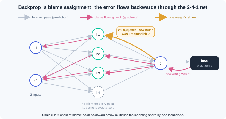
What the blame adds up to has a name from 0.7. The gradient — one slope per weight, each pointing where the loss rises — is the complete blame report. To improve, nudge every weight against its slope. And any single slope can be measured honestly with no theory: nudge the weight up by a tiny epsilon and read the loss, then nudge it down and read again. Rise over run gives the slope, exactly the trick module 0.7 played on a curve, now aimed at one weight inside a network.
There is a wrong way and a right way to use all this. The wrong way nudges weights at random and keeps whatever helped; with 17 weights the guesses mostly cancel, and with a million they never land. A quieter wrong way derives gradients on paper and trains on the unchecked formula, where one sign flip sends the whole network walking uphill. The right way follows the gradient and proves it first: every analytic gradient must match the numerical nudge to six decimal places. That check is this module's credibility moment, and WR-122 is the story of skipping it.
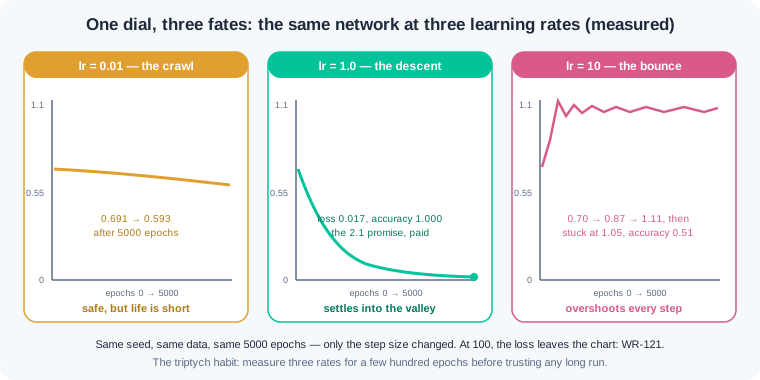
Gradient descent — the loop that repeats forward pass, blame, and a small downhill step — is all that training is. One full pass through the training data is an epoch — a lap, and you will run thousands of laps in seconds. The learning rate — the step size that scales every nudge — is the loop's one dangerous dial. Too small and the ball crawls for hours; too large and it bounces across the valley and lands higher than it started; reasonable and it settles. You will measure all three fates today, not take them on faith.
End on the honest deal. This is the last time you write a backward pass by hand: module 2.3 gives the same blame arithmetic to PyTorch's autograd, which runs it for any network, every time, without typos. You will trust that machine because today you built its insides and proved them against the nudge test. Choosing when to stop training, and the professional tricks around the learning rate, arrive in module 2.4.
Work inside ai-lab, NumPy only. This is one continuous session: each step builds on the previous one, so keep everything in a single file and run it top to bottom.
Step 1 — the honest slope: nudge one weight, watch the loss. Rebuild 2.1's XOR cloud exactly, give the 2-4-1 network small random weights, and measure one slope with no theory:
import numpy as np

rng = np.random.default_rng(2)                      # 2.1's XOR cloud, unchanged
pts = rng.uniform(0, 1, (200, 2)).round(2)
labels = ((pts[:, 0] > 0.5) != (pts[:, 1] > 0.5)).astype(int)
X, y = pts, labels.reshape(-1, 1)

def sigmoid(z): return 1 / (1 + np.exp(-z))

r = np.random.default_rng(24)                       # small random start
W1, b1 = r.normal(0, 0.5, (2, 4)), np.zeros(4)      # the 2-4-1 shapes from 2.1
W2, b2 = r.normal(0, 0.5, (4, 1)), np.zeros(1)

def loss():
    a1 = np.maximum(0, X @ W1 + b1)                 # the 2.1 forward pass
    p = np.clip(sigmoid(a1 @ W2 + b2), 1e-12, 1 - 1e-12)
    return -np.mean(y * np.log(p) + (1 - y) * np.log(1 - p))

p0 = sigmoid(np.maximum(0, X @ W1 + b1) @ W2 + b2)
print("random-init accuracy:", ((p0 > 0.5).astype(int) == y).mean())

eps = 1e-5
print(f"loss at w      : {loss():.8f}")
W1[1, 2] += eps;      up = loss()
W1[1, 2] -= 2 * eps;  down = loss()
W1[1, 2] += eps                                     # restore exactly
print(f"loss at w + eps: {up:.8f}")
print(f"loss at w - eps: {down:.8f}")
print(f"measured slope of W1[1,2]: {(up - down) / (2 * eps):.6f}")
Output: random-init accuracy: 0.47, then loss at w : 0.69100924, loss at w + eps: 0.69100928, loss at w - eps: 0.69100920, and measured slope of W1[1,2]: 0.003952. The random network is the 2.1 failure again — a coin flip. The loss is binary cross-entropy, 1.3's log loss on the sigmoid output, and the clip keeps log away from exact zero. Then the module's key move: raising W1[1,2] by 0.00001 raised the loss, lowering it lowered the loss, so this weight should move down. Slow but honest — two forward passes bought the true slope of one weight, and every gradient we compute from now on must answer to this test.
Step 2 — the backward pass: blame flowing back through the network. Instead of nudging 17 weights one by one, pass the error backwards once and collect every slope:
def forward(X):
    z1 = X @ W1 + b1
    a1 = np.maximum(0, z1)
    p = sigmoid(a1 @ W2 + b2)
    return z1, a1, p

def backward(X, y):
    z1, a1, p = forward(X)
    N = len(X)
    dz2 = (p - y) / N              # output's blame: how wrong, per point
    dW2 = a1.T @ dz2               # share for each hidden-to-output weight
    db2 = dz2.sum(axis=0)          # share for the output bias
    da1 = dz2 @ W2.T               # blame handed back to each hidden neuron
    dz1 = da1 * (z1 > 0)           # ReLU gate: silent neurons take no blame
    dW1 = X.T @ dz1                # share for each input-to-hidden weight
    db1 = dz1.sum(axis=0)
    return dW1, db1, dW2, db2

dW1, db1, dW2, db2 = backward(X, y)
print(f"backprop says W1[1,2]: {dW1[1, 2]:.6f}")
Output: backprop says W1[1,2]: 0.003952 — the same number Step 1 measured with nudges, now from algebra. Read the function downwards as blame flowing right to left. (p - y) is how wrong the output was, and sigmoid plus cross-entropy collapse to that clean difference. Each line after it multiplies the incoming blame by one local step of the chain rule: through W2, through the ReLU gate — a neuron that stayed silent for a point takes zero blame for it — and down to W1. Seven lines replace 34 forward passes.
Step 3 — the credibility moment: every gradient against the nudge test. Never trust a hand-written backward pass until it survives this:
def numerical(param, idx):
    param[idx] += eps;      up = loss()
    param[idx] -= 2 * eps;  down = loss()
    param[idx] += eps
    return (up - down) / (2 * eps)

rows = [("W1[0,0]", dW1[0, 0], numerical(W1, (0, 0))),
        ("b1[1]",   db1[1],    numerical(b1, (1,))),
        ("W2[0,0]", dW2[0, 0], numerical(W2, (0, 0))),
        ("W2[3,0]", dW2[3, 0], numerical(W2, (3, 0))),
        ("b2[0]",   db2[0],    numerical(b2, (0,)))]
print("weight     backprop    nudge")
for name, a, n in rows:
    print(f"{name:8s} {a: .6f}  {n: .6f}")
Output, side by side to six decimals:
weight     backprop    nudge
W1[0,0]  -0.001348   -0.001348
b1[1]    -0.027749   -0.027749
W2[0,0]  -0.007865   -0.007865
W2[3,0]   0.000000    0.000000
b2[0]     0.015729    0.015729
Every pair agrees to the last printed digit; extend the loop over all 17 numbers and the worst gap prints near 1e-11, float noise from WR-019 and nothing more. The backward pass is now proven, not believed. One row deserves a second look: W2[3,0] is exactly zero from both methods. Hidden neuron 4 happens to stay silent for all 200 points at this start — a 2.1 silent neuron — so it took part in nothing and earned zero blame. A zero gradient means "this weight changes nothing right now", and both methods agree on it independently.
Step 4 — gradient descent: the 2.1 promise, paid in full. Fresh start from the same seed, then thousands of downhill steps:
r = np.random.default_rng(24)
W1, b1 = r.normal(0, 0.5, (2, 4)), np.zeros(4)      # fresh random start
W2, b2 = r.normal(0, 0.5, (4, 1)), np.zeros(1)
lr = 1.0                                            # the step size

for epoch in range(1, 5001):
    dW1, db1, dW2, db2 = backward(X, y)
    W1 -= lr * dW1;  b1 -= lr * db1                 # every weight steps downhill
    W2 -= lr * dW2;  b2 -= lr * db2
    if epoch in (1, 100, 500, 1000, 3000, 5000):
        acc = ((forward(X)[2] > 0.5).astype(int) == y).mean()
        print(f"epoch {epoch:4d}  loss {loss():.4f}  accuracy {acc:.3f}")
Output, the loss actually falling, line by line: epoch 1 loss 0.6885 accuracy 0.525, then epoch 100 loss 0.4176 accuracy 0.865, epoch 500 loss 0.1371 accuracy 0.950, epoch 1000 loss 0.1095 accuracy 0.945, epoch 3000 loss 0.0286 accuracy 1.000, and finally epoch 5000 loss 0.0166 accuracy 1.000. This is the moment 2.1 promised. The network that scored 0.47 with random weights walked, on its own, to accuracy 1.000 on the XOR cloud — above the 0.99 the hand-set weights managed. Nobody told it about diagonal corners; the blame arithmetic found bends we set by intuition. Notice the loss keeps falling after accuracy tops out: past epoch 3000 the network is not changing answers, it is growing more confident in correct ones. And the whole 5000-epoch run takes seconds on a plain CPU.
Step 5 — the learning-rate triptych: measure all three fates. Same seed, same 5000 epochs, three step sizes:
def train(lr, epochs=5000):
    global W1, b1, W2, b2
    r = np.random.default_rng(24)
    W1, b1 = r.normal(0, 0.5, (2, 4)), np.zeros(4)
    W2, b2 = r.normal(0, 0.5, (4, 1)), np.zeros(1)
    for _ in range(epochs):
        dW1, db1, dW2, db2 = backward(X, y)
        W1 -= lr * dW1;  b1 -= lr * db1
        W2 -= lr * dW2;  b2 -= lr * db2
    return loss(), ((forward(X)[2] > 0.5).astype(int) == y).mean()

for lr_try in [0.01, 1.0, 10.0]:
    L, acc = train(lr_try)
    print(f"lr {lr_try:5}  final loss {L:.4f}  accuracy {acc:.3f}")
Output: lr 0.01 final loss 0.5931 accuracy 0.680, then lr 1.0 final loss 0.0166 accuracy 1.000, then lr 10.0 final loss 1.0535 accuracy 0.510. Three identical networks, three fates, decided by one number. At 0.01 the ball crawls: 5000 epochs moved the loss from 0.691 to 0.593, and full convergence would take lakhs of epochs. At 1.0 it settles into the valley. At 10.0 the first steps overshoot — print the early epochs and the loss bounces 0.70, 0.87, 1.11 — then it jams against a wall worse than where it started, with coin-flip accuracy. Push to 100 and the loss pins at 13.5 with the sigmoid saturated; without the clip in the loss it prints inf, then nan — WR-121's opening scene. The triptych habit — test three rates for a few hundred epochs before any long run — costs a minute and prevents that entire class of wasted evening.
Work inside ai-lab, NumPy only. Everything is seeded, so where a number is given your output must match it exactly.
The gradient-check ritual. Create blame_check.py. Rebuild the watch world exactly: XOR cloud from seed 2, network init from seed 24 with scale 0.5, zero biases, and the clipped cross-entropy loss. On paper first, write the chain of blame for the output bias b2 as three arrows (loss to p, p to z2, z2 to b2) and note the sigmoid-plus-cross-entropy shortcut: the blame arriving at z2 is (p - y) / N. Then implement backward and prove three named gradients against the numerical nudge with eps = 1e-5: print b2[0], W2[0,0], and b1[1] side by side to six decimals. Last, sabotage the code on purpose: change (p - y) to (y - p), rerun, and record what the table shows now. Check: the healthy table prints 0.015729, -0.007865, and -0.027749 twice each, matching in every printed digit; the sabotaged table flips the sign of every backprop column while the nudge column does not move; a closing comment explains why the nudge column is ground truth — it only ever runs forward passes, so no backward-pass bug can touch it.
Descend, then sabotage the descent. Create descend.py. Part one: train the seed-24 network with lr = 1.0 for 5000 epochs, recording loss and accuracy every 500 epochs into a list, and print the table at the end. Part two: change both update lines from -= to += (nothing else) and print the loss at epochs 1, 10, 25, and 50. Part three: restore -=, then initialise every weight matrix and bias to zeros instead of seed 24, train 2000 epochs, and print loss and accuracy at epochs 1, 100, and 2000, plus np.abs(dW1).max() at the final epoch. Write two comment lines: one explaining part two's climb, one explaining part three's flat line through the ReLU gate. Check: part one reaches accuracy 1.000 by epoch 3000 with loss below 0.03; part two climbs 0.693 to about 1.157 by epoch 10 and pins near 13.539 by epoch 25; part three sits at loss 0.6929 with accuracy 0.51 and prints a maximum dW1 blame of exactly 0.0; your comments name the flipped sign (uphill steps) and the silent-network plateau (zero hidden output means zero blame flows back, and 0.693 is the always-0.5 loss).
The learning-rate lab. Create lr_lab.py. Sweep five rates over the seed-24 network: [0.01, 0.1, 0.5, 1.0, 10.0], each trained 3000 epochs from the same fresh init. For every rate record final loss, final accuracy, and epochs-to-converge, defined as the first epoch where loss drops below 0.10 (record never if it does not). Print one table, one row per rate. Then choose the rate you would ship for tomorrow's retrain and defend it in a two-sentence comment that cites both a speed number and a stability observation from your own table. Check: the table matches these measured values — 0.01 gives loss 0.6429, accuracy 0.63, never; 0.1 gives 0.3168, 0.845, never; 0.5 gives 0.0486, 0.99, epoch 1320; 1.0 gives 0.0286, 1.0, epoch 991; 10.0 diverges to 1.0535, 0.51, never; your defence names 1.0 or 0.5 and rejects 10.0 with its measured row, not with a feeling.
Three training failures cover most of the pain in this module. Each has a War Room entry with the full diagnosis path:
- WR-121 — the loss that went to
nan. A learning rate set to 10 overshot the valley on every step, values overflowed within 20 epochs, and onenanpoisoned the rest of the run; the fix is the triptych habit, a 10x smaller rate, and knowing that gradient clipping is the professional guard arriving in 2.4. - WR-122 — the gradient with the wrong sign. A hand-derived gradient wrote
(y - p)for(p - y), so training climbed uphill smoothly and confidently; the numerical check caught it in one table, which is why the check is a ritual, not a ceremony. - WR-123 — the loss stuck at 0.693. Zero-initialised weights left every ReLU silent, so no blame could flow backwards and the loss pinned at ln 2, the always-0.5 score; the fix is small random init, and the lesson is to recognise 0.693 as an alarm number, not noise.
Training is gradient descent: run the forward pass, measure the loss, pass blame backwards, and step every weight a little downhill. Backpropagation computes each weight's blame share with the chain rule, and the numerical nudge check is the slow, honest ground truth it must match to six decimals. The learning rate sets the step size, and you measured all three fates: 0.01 crawled, 10 bounced into a wall, and 1.0 walked the XOR cloud from a coin flip to full accuracy. An epoch is one full pass through the data, and thousands of epochs finish in seconds on a plain CPU. This was the last backward pass you will write by hand, because module 2.3 gives the same arithmetic to autograd — and you will trust it, having built and checked it once yourself.
- UPI fraud models at Indian payment firms retrain on fresh transactions nightly. The retrain is exactly this loop — forward, loss, blame, nudge — walking yesterday's weights toward this week's scam patterns.
- Credit-scoring and crop-yield teams read loss curves before blaming data. A crawl, a bounce, or a 0.693-style plateau each points to a different fix, and you have produced all three on purpose.
- Every PyTorch or TensorFlow job in every company runs this module's blame arithmetic at scale; autograd is your seven-line backward pass generalised to any network shape.
Answer these before opening the gate assessment. Each question names its type.
type=output-prediction— A weight holds0.80, its gradient prints0.05, and the learning rate is0.5. Predict the weight's value after one gradient-descent update, and state whether this single step raises or lowers the loss.type=interpretation— A gradient-check table shows one row with backprop0.003952and nudge0.003952, and another row with backprop-0.041200and nudge0.041200. State what each row tells you, and name the first place in the backward pass you would inspect.type=debug— A training log prints loss0.6931, 0.6929, 0.6929, ...for 2000 epochs with accuracy pinned at0.51, andnp.abs(dW1).max()prints0.0. Name the initialisation mistake, the mechanism that keeps the gradients at zero, and the one-line fix.type=scenario-judgement— Demo tomorrow. A teammate sets the learning rate to 10 "so it converges ten times faster than 1.0". Give your judgement and the measured triptych evidence you would show, including where each of the two rates ends after 5000 epochs.type=trade-off— Numerical nudge gradients versus the hand-written backward pass, for this module's 17-weight network and for a million-weight network. Give one concrete advantage and one concrete cost of each method, and state the role this course assigns to each.
Explain to a friend who saw module 2.1's hand-set demo: how does the network find such weights on its own, and why does passing blame backwards tell every weight which way to move? Use at most 4 sentences, the ball-rolling-downhill picture, and no maths word beyond "slope". If your friend asks whether the machine guesses at random, you have your opening line ready.