PyTorch properly
Megha cleans loan data at an NBFC in Kota. Her mentor asks her to widen yesterday's tiny network from four hidden neurons to sixty-four. She spends the evening rewriting the backward pass by hand, and a sign error sends the loss climbing. Her mentor reads the screen, then deletes the whole page. "You built backprop once, so you have earned the machine that runs it for you. Prove the machine against your own numbers first." Tonight the same network trains in thirty lines of PyTorch.
- "Write a PyTorch training loop on paper" is a common fresher interview task at Indian AI teams, and tonight you learn to type it from memory.
- Every later module, from CNNs to LLM fine-tuning, runs on this same loop. Type it without thinking, and your attention goes to the model, not the plumbing.
- The whole module is CPU-only on an 8GB laptop. One pip install, and every training run here finishes in seconds or minutes.
PyTorch is NumPy with two superpowers, and you have already earned both. A tensor — PyTorch's n-dimensional array — behaves like the arrays you have used since 0.4: same shapes, same broadcasting, same slicing reflex. The bridge runs both ways: torch.from_numpy(a) wraps an array without copying, and t.numpy() hands it back. Memory is shared, so editing one side edits the other. The first superpower is speed on a GPU; the second matters more this week.
That second superpower is autograd — the engine that records every tensor operation and replays the chain backwards to produce every gradient. It is your 2.2 backward pass, generalised to any network shape and run without typos. Mark a tensor with requires_grad, compute a loss, call loss.backward(), and each weight's blame appears in its .grad. You will not take this on faith. Autograd must first reproduce the exact seed-24 gradients you computed by hand in 2.2, down to float noise.
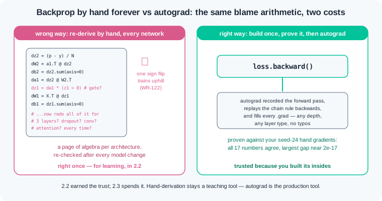
There is a wrong way and a right way to spend the skill 2.2 gave you. The wrong way re-derives the backward pass by hand for every new architecture — a page of algebra each time, where one sign flip walks the loss uphill (WR-122). The right way is the one this course planned: build backprop once, prove it, then hand the arithmetic to autograd forever. A second wrong way hides inside the loop itself: skip zero_grad and every old epoch's gradients pile into .grad. You will produce that failure on purpose today and learn its signature.
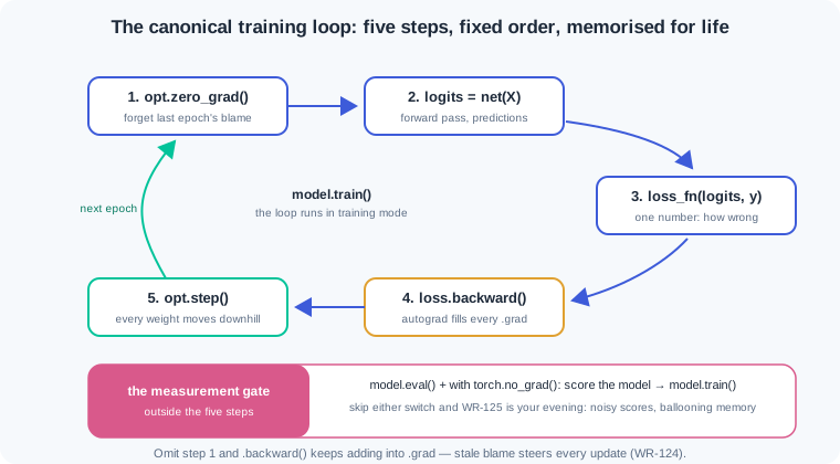
A network in PyTorch is a class built on nn.Module — the base class that collects layers, tracks their parameters, and moves them between devices. Your 2.1 net becomes eleven lines, and counting its parameters prints 17 — the same 17 weights you nudged by hand. Training that class is the canonical loop, five steps in fixed order: zero_grad, forward, loss, backward, step. An optimizer — the object that owns the update rule — performs the last step. SGD applies exactly 2.2's weight -= lr * grad, while Adam adapts a step size per weight; you will race them on the same problem.
Real datasets do not arrive in one gulp. A batch — a small slice of the data processed in one forward-backward pass — keeps memory flat on an 8GB laptop. The Dataset serves single examples, and the DataLoader — the loader that batches, shuffles and streams them — feeds the loop. Shuffling matters: sorted data teaches the network one city at a time, and it forgets the first while learning the last.
Two switches guard every measurement. model.train() and model.eval() flip layer behaviour, and torch.no_grad() tells autograd to stop recording, which saves memory during inference. Saving has its own rule: write the state_dict — the dictionary of a model's weights, keyed by layer name. Never pickle the whole model object; that file breaks the moment the class changes, a schema lesson module 4.1 will repeat.
The module ends honestly. On the small churn table, your network lands near 1.6's sklearn score, not above it. Deep nets earn their keep on images, sound and text; on 500 tabular rows, a logistic model with good features is a fair rival.
Work inside ai-lab. One-time setup: pip install torch==2.9.* — the CPU wheel, about 200 MB, is all this course needs. The pin is deliberate: every loss, gradient and accuracy printed in this phase was produced on this version, and a different torch build can shift the low decimals even with every seed fixed. Keep everything in one file per step and run top to bottom.
Step 1 — tensors and the NumPy bridge. Prove the two libraries share one worldview, then settle the device question once:
import numpy as np
import torch

a = np.array([[1.0, 2.0, 3.0], [4.0, 5.0, 6.0]])
t = torch.from_numpy(a)                     # no copy — same memory
print("numpy :", a.shape, a.dtype)
print("tensor:", t.shape, t.dtype)

t[0, 0] = 99.0                              # edit the tensor...
print("numpy sees it:", a[0])               # ...the array changed too
print("back again:", type(t.numpy()))

print("torch default:", torch.tensor([1.0]).dtype)

device = ("cuda" if torch.cuda.is_available()
          else "mps" if torch.backends.mps.is_available() else "cpu")
print("device:", device)
Output: numpy : (2, 3) float64, tensor: torch.Size([2, 3]) torch.float64, then numpy sees it: [99. 2. 3.], back again: <class 'numpy.ndarray'>, torch default: torch.float32, and on a course laptop device: cpu. Read the two dtype lines twice. from_numpy preserved float64, but fresh tensors default to float32 — two number formats that refuse to multiply together, and the ambush WR-126 documents. The device line is the pattern you write once at the top of every script: it prints cuda on an NVIDIA machine, mps on a newer Mac, cpu here — and .to(device) on the model and each batch makes the same script run on all three. Everything below runs on plain CPU in seconds.
Step 2 — the trust moment: autograd against your own hands. Rebuild 2.2's exact world — XOR cloud from seed 2, weights from seed 24 — wrap it in tensors, and let autograd answer for itself:
rng = np.random.default_rng(2)
pts = rng.uniform(0, 1, (200, 2)).round(2)
labels = ((pts[:, 0] > 0.5) != (pts[:, 1] > 0.5)).astype(int)
X = torch.from_numpy(pts)
y = torch.from_numpy(labels.reshape(-1, 1).astype(np.float64))

r = np.random.default_rng(24)                        # 2.2's init, same order
W1 = torch.from_numpy(r.normal(0, 0.5, (2, 4))).requires_grad_()
b1 = torch.zeros(4, dtype=torch.float64, requires_grad=True)
W2 = torch.from_numpy(r.normal(0, 0.5, (4, 1))).requires_grad_()
b2 = torch.zeros(1, dtype=torch.float64, requires_grad=True)

logits = torch.relu(X @ W1 + b1) @ W2 + b2           # the 2.1 forward pass
loss = torch.nn.functional.binary_cross_entropy_with_logits(logits, y)
loss.backward()                                      # the whole of 2.2, one line

print(f"loss: {loss.item():.8f}")
rows = [("W1[1,2]", W1.grad[1, 2],  0.003952), ("W1[0,0]", W1.grad[0, 0], -0.001348),
        ("b1[1]",   b1.grad[1],    -0.027749), ("W2[0,0]", W2.grad[0, 0], -0.007865),
        ("W2[3,0]", W2.grad[3, 0],  0.000000), ("b2[0]",   b2.grad[0],     0.015729)]
print("weight     autograd    2.2 by hand")
for name, g, hand in rows:
    print(f"{name:8s} {g.item(): .6f}  {hand: .6f}")
Output: loss: 0.69100924 — 2.2's Step 1 loss to the last digit — then six rows where the autograd column matches the hand column in every printed digit, including W2[3,0] at exactly zero for the silent neuron. Extend the comparison across all 17 numbers against your 2.2 backward function and the largest gap prints near 2e-17, tighter than the 1e-11 nudge-test standard, because both sides ran the same float64 arithmetic. Note what you did not write: no dz2, no ReLU gate, no chain of blame — backward() recorded the forward pass and replayed it in reverse. The loss line also settles a naming question: binary_cross_entropy_with_logits takes raw scores before the sigmoid. Feeding a saturated sigmoid output to plain BCE loses the true loss — at logit 50 it reports a clamped 100.0 where the logits version reports the exact 50.0 — which is why the fused loss is the professional default.
Step 3 — the 2.1 net as a class. nn.Module turns loose matrices into a named, countable, portable model:
import torch.nn as nn

class TinyNet(nn.Module):
    def __init__(self):
        super().__init__()
        self.hidden = nn.Linear(2, 4)       # W1 and b1, managed
        self.out = nn.Linear(4, 1)          # W2 and b2, managed

    def forward(self, x):
        return self.out(torch.relu(self.hidden(x)))

def seed24_init(model):                     # 2.2's exact starting weights
    r = np.random.default_rng(24)
    w1, w2 = r.normal(0, 0.5, (2, 4)), r.normal(0, 0.5, (4, 1))
    with torch.no_grad():
        model.hidden.weight.copy_(torch.from_numpy(w1.T))   # note the .T
        model.out.weight.copy_(torch.from_numpy(w2.T))
        model.hidden.bias.zero_(); model.out.bias.zero_()

net = TinyNet().double()
seed24_init(net)
for name, p in net.named_parameters():
    print(f"{name:14s} shape {tuple(p.shape)}  numel {p.numel()}")
print("total parameters:", sum(p.numel() for p in net.parameters()))
with torch.no_grad():
    p0 = torch.sigmoid(net(X))
print(f"random-init accuracy: {((p0 > 0.5).double() == y).double().mean().item():.2f}")
Output: four parameter rows — hidden.weight shape (4, 2) numel 8, hidden.bias (4,) numel 4, out.weight (1, 4) numel 4, out.bias (1,) numel 1 — then total parameters: 17 and random-init accuracy: 0.47. Seventeen parameters: the same count you gradient-checked in 2.2, now tracked automatically, and the same coin-flip start. One trap worth the comment: nn.Linear(2, 4) stores its weight as (4, 2) — out-features by in-features — so porting 2.2's (2, 4) matrix needs the transpose. Skip the .T and the copy still succeeds on this square-free shape mismatch pair only by luck of dimensions; audit shapes at every boundary. The forward method returns logits, not probabilities, because Step 2's fused loss wants raw scores; the sigmoid appears only at prediction time.
Step 4 — the canonical loop, and the 2.2 promise repaid. Five steps in fixed order, memorised for life — then proof that PyTorch walks the exact path your NumPy code walked:
net = TinyNet().double()
seed24_init(net)
loss_fn = nn.BCEWithLogitsLoss()
opt = torch.optim.SGD(net.parameters(), lr=1.0)      # 2.2's rule, 2.2's rate

for epoch in range(1, 5001):
    opt.zero_grad()                # 1. forget last epoch's gradients
    logits = net(X)                # 2. forward
    loss = loss_fn(logits, y)      # 3. loss
    loss.backward()                # 4. backward — autograd fills .grad
    opt.step()                     # 5. every weight steps downhill
    if epoch in (1, 100, 500, 1000, 3000, 5000):
        net.eval()
        with torch.no_grad():
            L = loss_fn(net(X), y).item()
            acc = ((torch.sigmoid(net(X)) > 0.5).double() == y).double().mean()
        net.train()
        print(f"epoch {epoch:4d}  loss {L:.4f}  accuracy {acc.item():.3f}")
Output, line by line: epoch 1 loss 0.6885 accuracy 0.525, epoch 100 loss 0.4176 accuracy 0.865, epoch 500 loss 0.1371 accuracy 0.950, epoch 1000 loss 0.1095 accuracy 0.945, epoch 3000 loss 0.0286 accuracy 1.000, epoch 5000 loss 0.0166 accuracy 1.000. Put 2.2's Step 4 table beside this one: every loss and every accuracy matches to the printed digit. Same seed, same data, same arithmetic — different engine. That is the whole argument for trusting PyTorch, and it took about thirty lines. The measurement block inside the if is the eval ritual: net.eval() plus torch.no_grad(), then back to net.train() — pointless-looking on this tiny net, but dropout and batch norm arrive in 2.4 and betray anyone without the habit (WR-125). Say the five steps aloud once: zero_grad, forward, loss, backward, step.
Step 5 — the bug you must recognise on sight. Same net, same rate, one line deleted:
net = TinyNet().double()
seed24_init(net)
opt = torch.optim.SGD(net.parameters(), lr=1.0)

for epoch in range(1, 501):
    loss = loss_fn(net(X), y)      # zero_grad() is missing — on purpose
    loss.backward()
    opt.step()
    if epoch in (1, 10, 50, 100, 200, 500):
        with torch.no_grad():
            L = loss_fn(net(X), y).item()
        g = net.hidden.weight.grad.abs().max().item()
        print(f"epoch {epoch:3d}  loss {L:.4f}  max|grad| {g:.3f}")
Output: epoch 1 loss 0.6885 max|grad| 0.032, epoch 10 loss 0.6306 max|grad| 0.187, epoch 50 loss 0.4094 max|grad| 0.484, epoch 100 loss 0.5406 max|grad| 0.440, epoch 200 loss 0.3936 max|grad| 0.652, epoch 500 loss 0.3561 max|grad| 0.827. Read it against Step 4's healthy run. The buggy loop looks faster at first — 0.4094 at epoch 50 against 0.5945 — because summed gradients act like a growing learning rate. Then it betrays: up to 0.5406 at epoch 100 while the clean run passed 0.4176, and by epoch 500 it wanders at 0.3561 while the clean run sits at 0.1371 on its way to full accuracy. The tell is the third column: .backward() adds into .grad by design, so the stored gradient grows 0.032 to 0.827 while a healthy run's gradients shrink toward zero. Falling-then-wandering loss plus growing gradients is WR-124's signature; on bigger nets the same bug ends in nan. The fix is not cleverness, it is the memorised order.
Step 6 — the churn world, batched, and an honest scoreboard. Phase 1's Ludhiana table becomes tensors, a DataLoader feeds the loop, and the network faces 1.6's logistic pipeline:
import pandas as pd
from torch.utils.data import TensorDataset, DataLoader
from sklearn.model_selection import train_test_split
from sklearn.preprocessing import StandardScaler

rng = np.random.default_rng(42)                      # 1.6's world, unchanged
n = 500
snapshot = pd.Timestamp("2026-06-30")
customers = pd.DataFrame({
    "city": rng.choice(["Ludhiana", "Jalandhar", "Amritsar",
                        "Patiala", "Bathinda"], size=n),
    "monthly_income": rng.integers(18000, 120000, size=n),
    "orders_last_90d": rng.poisson(6, size=n),
    "avg_order_value": rng.integers(120, 900, size=n)})
customers["last_order_date"] = snapshot - pd.to_timedelta(
    rng.integers(1, 120, size=n), unit="D")
spend_share = (customers["avg_order_value"] * customers["orders_last_90d"]
               / 3) / customers["monthly_income"]
days_since = (snapshot - customers["last_order_date"]).dt.days
salary_week = (customers["last_order_date"].dt.day <= 7).astype(int)
risk = (-3.0 + 0.05 * days_since - 25 * spend_share
        - 1.3 * salary_week - 0.15 * customers["orders_last_90d"])
customers["churned"] = (rng.random(n) < 1 / (1 + np.exp(-risk))).astype(int)
customers["days_since_last_order"] = days_since
customers["spend_share"] = spend_share
customers["salary_week_order"] = salary_week

feats = ["monthly_income", "orders_last_90d", "avg_order_value",
         "days_since_last_order", "spend_share", "salary_week_order"]
X_train, X_test, y_train, y_test = train_test_split(
    customers[feats], customers["churned"],
    test_size=0.25, random_state=42, stratify=customers["churned"])

scaler = StandardScaler().fit(X_train)               # train rows only, 1.7's law
Xtr = torch.tensor(scaler.transform(X_train), dtype=torch.float32)
Xte = torch.tensor(scaler.transform(X_test), dtype=torch.float32)
ytr = torch.tensor(y_train.values, dtype=torch.float32).reshape(-1, 1)
yte = torch.tensor(y_test.values, dtype=torch.float32).reshape(-1, 1)

torch.manual_seed(7)
train_dl = DataLoader(TensorDataset(Xtr, ytr), batch_size=32, shuffle=True)
print("batches per epoch:", len(train_dl))
xb, yb = next(iter(train_dl))
print("one batch:", xb.shape, yb.shape, xb.dtype)

model = nn.Sequential(nn.Linear(6, 16), nn.ReLU(), nn.Linear(16, 1))
loss_fn = nn.BCEWithLogitsLoss()
opt = torch.optim.Adam(model.parameters(), lr=0.001)

for epoch in range(1, 201):
    model.train()
    for xb, yb in train_dl:                          # one batch at a time
        opt.zero_grad()
        loss = loss_fn(model(xb), yb)
        loss.backward()
        opt.step()
    if epoch in (1, 50, 100, 200):
        model.eval()
        with torch.no_grad():
            pred = (torch.sigmoid(model(Xte)) > 0.5).float()
        print(f"epoch {epoch:3d}  test accuracy {(pred == yte).float().mean().item():.2f}")

caught = int(((pred == 1) & (yte == 1)).sum().item())
print(f"neural net    accuracy: {(pred == yte).float().mean().item():.2f}"
      f"   caught: {caught} of {int(yte.sum().item())}")
print("1.6 logistic  accuracy: 0.83   caught: 27 of 39")
Output: batches per epoch: 12, then one batch: torch.Size([32, 6]) torch.Size([32, 1]) torch.float32, then epoch 1 test accuracy 0.69, epoch 50 test accuracy 0.80, epoch 100 test accuracy 0.78, epoch 200 test accuracy 0.79, then the scoreboard — neural net accuracy: 0.79 caught: 24 of 39 against 1.6 logistic accuracy: 0.83 caught: 27 of 39. Read the honest parts in order. The DataLoader cut 375 training rows into 12 shuffled batches of 32, so the loop gained an inner for — the only structural change from Step 4, and the one that scales to tables too big for memory. The batch print is the WR-126 audit: shapes and dtype checked once at the boundary, before any training. Epoch 1 sits at the 0.69 do-nothing baseline; by epoch 50 the net has learned what the engineered features offer, and further epochs drift on a 125-row test set. And the scoreboard: the network lost to 1.6's plain logistic pipeline. Deep nets do not automatically beat simpler models on small tabular data — the features carried the signal, and both models read the same features. This result is worth more than a win: you now know the claim "we need deep learning" is a hypothesis to test against a baseline, not a reflex. Exact float32 digits may differ slightly across machines; the ranking should not.
Work inside ai-lab with your tvenv (or any venv) holding torch, numpy, pandas and scikit-learn. The XOR-cloud drills run in float64 and are seeded, so given digits must match exactly; the churn project runs in float32, where tiny platform differences are allowed and stated.
If your numbers are close but not identical, triage in a fixed order before touching your code. Everything off by a little — every value drifting in the last decimal or two — points at a library version: run pip show torch, compare it with the pinned install line, and match the pin, because the printed numbers were produced on that version. One number wildly off while the rest agree points at stale state: restart from a fresh kernel or a fresh python and run the file top to bottom, since seeded draws only reproduce when they happen in the same order from a clean start. Only when both checks pass and the numbers still disagree should you suspect your own logic — diff your script line by line against the printed code.
Port your 2.2 net and prove nothing changed. Create torch_port.py. Part one: rebuild the XOR cloud from seed 2 and the seed-24 weights (one rng, W1 drawn before W2, biases zero), wrap everything with torch.from_numpy, mark the four parameter tensors with requires_grad, run the forward pass with torch.relu and matrix multiply, take binary_cross_entropy_with_logits, and call loss.backward(). Print the loss to 8 decimals, then a six-row table — W1[1,2], W1[0,0], b1[1], W2[0,0], W2[3,0], b2[0] — with autograd's number beside 2.2's hand value. Part two: paste your 2.2 NumPy backward into the same file, run it on identical inputs, and print the largest absolute gap across all 17 gradients. Part three: build the TinyNet class, copy the same weights in (mind the transpose), and train 5000 epochs of full-batch SGD at rate 1.0, printing loss and accuracy at epochs 1, 100, 500, 1000, 3000, 5000. Check: the loss prints 0.69100924; the table matches 2.2 in every digit — 0.003952, -0.001348, -0.027749, -0.007865, 0.000000, 0.015729; the largest gap prints below 1e-12; the training table matches 2.2's run line for line, ending at loss 0.0166, accuracy 1.000; a closing comment states why nn.Linear(2, 4) needed w1.T (weights stored out-features by in-features).
The optimizer derby. Create optimizer_derby.py. Four runs on the same TinyNet, each from a fresh seed-24 init, full batch, 5000 epochs: SGD at rate 1.0, SGD at 0.1, Adam at 0.01, Adam at 0.5. After each configured epoch — 100, 500, 1000, 3000, 5000 — record the loss measured under torch.no_grad(), and record final accuracy. Print one table, one row per optimizer. Then write a three-sentence verdict in comments: which configuration you would ship for this problem, which numbers from your own table support it, and what Adam at 0.5 proves about the claim "Adam removes learning-rate tuning". Check: SGD 1.0 reproduces the canonical run ending at 0.0166 with accuracy 1.000; SGD 0.1 crawls to 0.3158 and accuracy 0.840; Adam 0.01 ends lowest at 0.0046 with accuracy 1.000; Adam 0.5 pins near 0.3157 with accuracy 0.840, matching SGD 0.1's plateau; the verdict cites at least three numbers from the table and names the lesson that Adam adapts step sizes but is not immune to a bad base rate.
Churn, as tensors — the full project. Create churn_torch.py. Rebuild 1.6's Ludhiana world exactly: seed 42, n=500, columns drawn in the lesson's order, the three engineered features added, the usual split (test 0.25, seed 42, stratified). Fit StandardScaler on training rows only, convert to float32 tensors with labels reshaped to (-1, 1), call torch.manual_seed(7), then build a DataLoader (batch 32, shuffled) and the model nn.Sequential(nn.Linear(6, 16), nn.ReLU(), nn.Linear(16, 1)). Train 200 epochs with Adam at 0.001 and BCEWithLogitsLoss, following the canonical loop inside the batch loop. Measure test accuracy at epochs 1, 50, 100, 200 — every measurement inside model.eval() plus torch.no_grad(), returning to model.train() after. Print a final scoreboard: your accuracy, recall and caught-of-39 beside 1.6's row (accuracy 0.83, recall 0.69, caught 27 of 39). Close with two sentences: one comparing the two models honestly, one explaining what breaks if the eval ritual is skipped once dropout arrives in 2.4. Check: batches per epoch prints 12 and one batch prints shapes (32, 6) and (32, 1) in float32; epoch-1 accuracy sits at the do-nothing baseline near 0.69; final accuracy lands between 0.77 and 0.81 (reference run: 0.79, recall 0.62, caught 24 of 39) — below the logistic pipeline; your sentences state that the network did not beat 1.6's model on this small table and name both model.eval() and torch.no_grad() as the measurement guard.
The state_dict round trip. Create save_load.py. Train your TinyNet from exercise 1 for 500 epochs, then: print list(net.state_dict().keys()); save with torch.save(net.state_dict(), "xor_net.pt"); build a brand-new TinyNet().double() and confirm its fresh predictions differ from the trained net's; call load_state_dict on the saved file; put both models in eval mode and print the maximum absolute gap between their predictions on the full cloud, plus the saved file's size in bytes. Then demonstrate the wrong way by name: torch.save(net, "whole_model.pt") pickles the entire object, and a comment must explain why it is refused in this course — the pickle binds to the class's import path and source, so any refactor or rename breaks loading, which is 4.1's schema lesson wearing PyTorch clothes. Bonus: move TinyNet into a differently named module, reload both files, and record which one survives. Check: the keys print exactly ['hidden.weight', 'hidden.bias', 'out.weight', 'out.bias']; the prediction gap after reload prints 0.0; the file size is near 2.5 KB — seventeen float64 weights plus names, nothing else; the comment names the import-path fragility and names state_dict as the shippable artifact.
Three PyTorch failures cover most of this module's pain. Each has a War Room entry with the full diagnosis path:
- WR-124 — the gradients that never forgot. A loop without
zero_gradtrained fast, then wandered:.backward()adds into.gradby design, so stale blame from every past epoch steered each step; the fix is the five-step canonical order, memorised, and the tell is stored gradients growing while the loss drifts. - WR-125 — the eval-mode betrayal. Validation run in training mode and without
torch.no_grad(): scores turned noisy once dropout arrived, and memory ballooned because autograd recorded a graph for every eval batch; the fix is the two-switch ritual —model.eval()withno_grad, then back tomodel.train(). - WR-126 — the shape and dtype ambush. A float64 NumPy tensor met float32 weights and crashed loudly, but the dangerous cousin was silent: an
(N,)target against an(N, 1)prediction broadcast into an N-by-N comparison and printed a confident, meaningless accuracy; the fix is a dtype-and-shape audit at the tensor boundary, every project.
PyTorch tensors are NumPy arrays with autograd attached, and the bridge between the two runs both ways without copying. Autograd matched your hand-computed seed-24 gradients to float noise, and the canonical loop then repeated 2.2's whole training table digit for digit. The loop is five steps in fixed order — zero_grad, forward, loss, backward, step — and skipping the first step lets stale gradients pile up until training wanders. DataLoader feeds the loop in shuffled batches, model.eval() with torch.no_grad() guards each measurement, and the state_dict is the only file you save. On the churn table the network scored 0.79 against the pipeline's 0.83: on small tables, deep learning is a rival to test, not a rescue.
- UPI fraud teams at Indian banks and fintechs run this loop nightly. A DataLoader streams fresh transactions, the five steps run, and a state_dict checkpoint lands before the morning shift.
- Shared GPU servers at Indian startups can vanish mid-run when spot prices spike. The team that saved a state_dict every epoch resumes in minutes; the team that pickled whole models rebuilds.
- Every open model you will meet in Phase 3 ships as a state_dict. Hugging Face checkpoints load into a model class the same way your exercise 4 file does it.
Answer these before opening the gate assessment. Each question names its type.
type=output-prediction— After one training step, a weight's.gradholds0.05. The same batch is run forward again,loss.backward()is called again, and nozero_gradhappened in between. Predict the value now stored in.grad, and the size of the next SGD step at learning rate 1.0 relative to a correct one.type=debug— A script wraps NumPy features withtorch.from_numpyand feeds them to a freshnn.Linearmodel. It crashes withRuntimeError: mat1 and mat2 must have the same dtype, but got Double and Float. Name the cause on each side of the multiplication and the one-line fix at the tensor boundary.type=interpretation— Step 6's scoreboard reads: neural net 0.79, logistic pipeline 0.83, both on the same engineered features. A teammate concludes "PyTorch is worse than sklearn". Give the correct reading of the two numbers, and state what the result says about where deep nets earn their keep.type=scenario-judgement— Before a demo, a teammate proposes saving withtorch.save(model)because "one line restores everything, no class needed". Judge the proposal, name the failure it invites during any refactor, and state what you would save instead and what must travel with it.type=trade-off— Full-batch training (Step 4) versus DataLoader mini-batches (Step 6), for the 500-row churn table and for a 12-lakh-row transaction table. Give one concrete advantage and one concrete cost of each approach, and state which one each table demands.
Explain to a friend who finished 2.2's hand-written backprop: why can they now trust loss.backward() to do that work, and what do the five steps of the training loop each do? Use at most 4 sentences, name the proof (autograd matched their own seed-24 gradients), and keep the loop order exact — zero_grad, forward, loss, backward, step. If they ask "then why did we do it by hand at all", your first sentence is the answer.