The maths you will actually use
Tuesday, 11 am. Sneha joins an agritech startup in Indore that predicts crop yields. Her lead shares a model paper full of Greek symbols and asks what it is doing. Her stomach drops — she scraped through college maths and has feared it ever since. Then her senior opens a notebook and turns the scariest formula into four short lines of NumPy that print numbers she can read. Same maths, different door. Today you enter through that door: pictures first, then code, no proofs.
- The maths behind AI is a short list, and this module covers the whole working set for Phases 1 to 3.
- Interviewers test intuition — why a dot product measures similarity — far more often than they test proofs.
- Freshers who can read a slope, a chance, and a spread can debug models; freshers who fear them can only guess.
Here is the secret nobody told you in college. AI does not use most of the maths syllabus. It runs on a small working set: vectors, dot products, matrices, slopes, chance, and logs. You will meet each one three ways — a picture, one plain sentence, and a few lines of NumPy you can run. No proofs appear anywhere in this module.
There is a wrong way and a right way to face a formula. The wrong way reads it symbol by symbol, tries to memorise it, and panics when one Greek letter is unfamiliar. The right way asks two questions: what shape goes in, and what shape comes out. Then it translates the formula into code and pokes it with real numbers. A formula you can run is a function, not a threat.
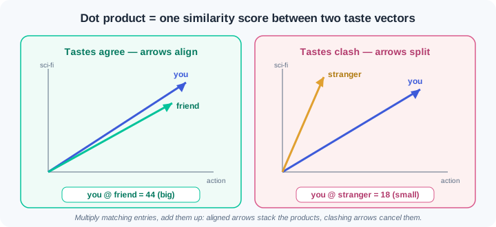
Start with the vector — a list of numbers that describes one thing. Your movie tastes can be a vector: one number per genre. The dot product — multiply matching entries, then add the results — turns two vectors into a single score. When two vectors point the same way, the score is large; when they disagree, it shrinks. That one score powers every "people like you also watched" feed.
A matrix is a grid of numbers that works like a machine: a vector goes in, a different vector comes out. The shape rule from module 0.4 tells you what fits: a (2, 3) matrix eats a vector of 3 and produces a vector of 2. Every layer of a neural network is exactly this machine, applied again and again. Nobody computes these by hand at work — the skill is predicting the output shape.
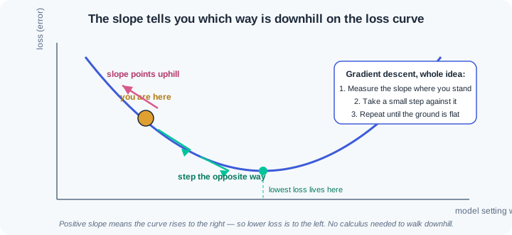
Now picture a loss curve: model error on the y-axis, one model setting on the x-axis. The slope at your current point tells you which way the curve rises. The gradient — the slope that points uphill — is the compass of machine learning. To improve, step the opposite way: downhill, where the error is lower. Repeat small steps, and you have gradient descent, the engine you will meet properly in Phase 2.
Probability — a number between 0 and 1 that measures how likely something is — is how code talks about chance. Conditional thinking asks a sharper question: given what I already know, what are the chances now? Calibration matters more than confidence: a model that says 90% should be right about nine times out of ten. A fraud model that shouts 99% and is wrong half the time is worse than useless.
A pile of data has a shape, and two numbers sketch it fast. The mean marks the centre. The variance — the average squared distance from the mean — measures the spread around it. Two delivery routes can share a mean of 30 minutes while one swings wildly and the other barely moves. The shape of the whole pile is its distribution, and reading distributions is daily work for analysts.
One last tool: the logarithm — the power you raise a base to in order to reach a number. Logs have one superpower you will use constantly: they turn multiplication into addition. Multiply thousands of small chances and the result collapses to zero; add their logs and the answer stays healthy. That is why nearly every loss function in machine learning has a log inside it.
Watch the full flow once before you try it. Every demo is under six lines — type it, run it, then change a number and watch what moves. That habit of poking is the whole method.
Step 1 — the dot product as a similarity score. Three users rate four genres, 0 to 5:
import numpy as np

you      = np.array([5, 1, 4, 2])   # action, romance, sci-fi, drama
friend   = np.array([4, 2, 5, 1])
stranger = np.array([1, 5, 0, 4])
print(you @ friend, you @ stranger)
Output: 44 18. The @ operator multiplies matching entries and adds them: 5×4 + 1×2 + 4×5 + 2×1 = 44. Your friend's high sci-fi rating lines up with yours, so the products stack up. The stranger loves what you skip, so the score sinks to 18. Recommendation feeds compute this exact score between you and crores of other users, then rank.
Step 2 — a matrix is a machine. Feed a vector in, read a vector out:
M = np.array([[2, 0],
              [0, 3]])
v = np.array([1, 1])
print(M @ v)
print(M.shape, v.shape, (M @ v).shape)
Output: [2 3] then (2, 2) (2,) (2,). This machine stretched the first entry by 2 and the second by 3. The shape line is the professional reading: a (2, 2) matrix ate a length-2 vector and returned a length-2 vector. Every neural network layer is this pattern with far bigger shapes — and you will read it the same way.
Step 3 — the slope of a loss curve, numerically. No calculus, one subtraction:
def loss(w):
    return (w - 3) ** 2 + 1

w, h = 5.0, 1e-5
slope = (loss(w + h) - loss(w - h)) / (2 * h)
print(round(slope, 4))
print(loss(w), loss(w - 0.1 * slope))
Output: 4.0, then 5.0 3.5600000000484577. Nudge w both ways, divide rise by run — that fraction is the slope, no formula sheet needed. It is positive, so the curve rises to the right, which means downhill is to the left. One small step against the slope drops the loss from 5.0 to about 3.56; loop that step and you have gradient descent. (The trailing ...0484577 digits are float noise — WR-019 explains why they appear.)
Step 4 — chance settles as the sample grows. Flip a fair coin one lakh times:
rng = np.random.default_rng(0)
flips = rng.integers(0, 2, size=100_000)
for n in [10, 100, 10_000, 100_000]:
    print(n, flips[:n].mean())
Output: 10 0.4, 100 0.56, 10000 0.503, 100000 0.49958. Ten flips of a fair coin said 0.4 — wildly off, and completely normal. The estimate only settles near the true 0.5 as the sample grows. The seed makes your run match this one exactly; delete it and the small-sample numbers jump around on every run. Both traps — tiny samples and missing seeds — are WR-021.
Step 5 — mean and variance in one glance. Two delivery routes, same average:
route_a = np.array([29, 30, 31, 30, 30])
route_b = np.array([5, 55, 30, 10, 50])
print(route_a.mean(), route_b.mean())
print(route_a.var(),  route_b.var())
Output: 30.0 30.0 then 0.4 410.0. The mean alone claims the routes are identical. The variance exposes the truth: route A is dependable, route B is chaos with the same average. When anyone quotes you an average — delivery time, salary, crop yield — ask for the spread before deciding anything.
Step 6 — logs turn products into sums. Multiply 6,000 chances, then rescue them:
p = np.array([0.9, 0.5, 0.6] * 2000)   # 6,000 chances
print(p.prod())
print(np.log(p).sum())
print(np.log(0.9 * 0.5), np.log(0.9) + np.log(0.5))
Output: 0.0, then -2618.6666399675246, then two identical values near -0.7985. The true product is a real, tiny number — but it fell below the smallest value a float can hold and flattened to exact zero. The summed logs carry the same information comfortably, because log(a×b) = log(a) + log(b), which the last line proves. This silent collapse is WR-020, and log space is the standard rescue built into every loss you will meet.
Do these inside your ai-lab environment from module 0.1, with NumPy installed. Each exercise ends with a check — you are done only when the check passes.
Taste-match engine. Create taste.py. Write your own movie-taste vector: five genres, each rated 0 to 5. Invent vectors for three friends with different personalities — one near-twin, one opposite, one mixed. Compute your dot product with each friend using @ and print the three scores ranked, highest first, with names. Then build the opposite friend by hand as 5 - twin and confirm their score lands lowest. Check: python taste.py prints three labelled scores in descending order, and a one-line comment in the file explains why the twin scored highest in terms of matching entries.
Walk downhill by hand. Create downhill.py. Define loss(w) as (w - 4) ** 2 + 2. Write a slope helper using (loss(w + h) - loss(w - h)) / (2 * h) with h = 1e-5. Starting from w = 9.0, take 25 steps of w = w - 0.1 * slope, printing step number, w, and loss(w) each time. Then rerun with the step factor changed from 0.1 to 1.1 and watch the walk explode instead of settling. Check: the first run ends with w within 0.1 of 4 and loss near 2; the second run's loss grows every step; one sentence in maths-notes.md explains why the step size flipped the outcome.
Chance lab. Create chance.py. Simulate 100,000 dice rolls with np.random.default_rng(42). Print the fraction of sixes after 10, 100, 10,000, and 100,000 rolls and watch it settle near 0.1667. Then answer a conditional question with a boolean mask: among rolls greater than 3, what fraction are even? Compare your simulated value to the pen-and-paper answer of 2/3. Finally, reproduce WR-021 on purpose: remove the seed, run the script twice, and record how the 10-roll fractions disagree between runs while the 100,000-roll fractions barely move. Check: the simulated conditional fraction lands within 0.01 of 0.667, and maths-notes.md records the two unseeded 10-roll values side by side.
Break the number line, then rescue it with logs. Create rescue.py. First reproduce WR-019: print 0.1 + 0.2 == 0.3, print the sum with f"{0.1 + 0.2:.20f}", then fix the comparison with np.isclose. Next reproduce WR-020 both ways: print np.exp(1000.0) (note the overflow warning and inf), then multiply 6,000 chances drawn with rng.uniform(0.3, 0.9, 6000) and watch the product print 0.0. Rescue the product with np.log(...).sum() and show a healthy finite number. Finish by proving the log law on two small numbers: np.log(a * b) versus np.log(a) + np.log(b). Check: the script prints each broken result directly above its fixed version, and two sentences in maths-notes.md explain why logs saved the product.
Three failures cover most first-month maths-in-code pain. Each has a War Room entry with the full diagnosis path:
- WR-019 —
0.1 + 0.2 == 0.3printsFalse. Floats store decimals approximately, so equality checks on computed values break — and probabilities sum to 0.9999999 instead of 1. - WR-020 —
infand0.0out of nowhere.np.expof a big number overflows to infinity, and a product of thousands of chances silently underflows to zero. Logs are the standard rescue. - WR-021 — every run gives a different answer. No seed was set, so each run is a new experiment — or a confident conclusion rests on a sample far too small to mean anything.
AI runs on a small maths toolkit: vectors, dot products, matrices, slopes, chance, and logs. A dot product multiplies matching entries and adds them, and a big score means two vectors point the same way. A matrix is a machine that turns one vector into another, and the slope of a loss curve tells you which way is downhill. Probability puts a number between 0 and 1 on chance, while mean and variance describe a data pile's centre and spread. When many chances multiply into numbers too small for a float, take logs and add instead.
- Recommendation feeds on Indian OTT and shopping apps score your taste vector against crores of users with dot products — exercise 1 at industrial scale.
- Credit scoring at banks and UPI fintechs ships calibrated chances, because a lender acting on a 90% score needs it right about nine times in ten.
- Crop and weather advisories report means, variances, and distributions of rainfall, since an average alone would mislead a farmer badly in a swingy season.
Answer these before opening the gate assessment. Each question names its type.
type=output-prediction— Givena = np.array([2, 0, 1])andb = np.array([3, 5, 4]), predict exactly whata @ bprints, then state what a much smaller score would have told you about the two vectors.type=debug— A teammate's fraud script multiplies 8,000 per-transaction chances and prints0.0, so the alert never fires. Name the cause and the one-line change you would make.type=interpretation— At the current settingw = 2, the numerical slope of the loss prints-6.0. Which direction shouldwmove to reduce the loss, and what does the sign tell you about the curve at that point?type=scenario-judgement— A teammate tests the model on 30 rows, gets 97% accuracy, and wants to announce the number to the client today. Give your judgement and the one-sentence reason you would offer.type=trade-off— Storing raw probabilities versus storing their logs in a scoring pipeline: give one concrete advantage and one concrete cost of each choice.
Explain to a friend who fears maths: how does a shopping app decide that you and a stranger have similar taste, and why is one multiply-and-add score enough to power the whole feed? Use at most 4 sentences, no symbols, and no jargon beyond "list of numbers". If your friend smiles instead of flinching, you own this module.