Unsupervised learning
Varun is the first data analyst at a kirana-delivery startup in Warangal. The founder slides a laptop across the table: eight hundred customers, five columns, and no label anywhere. Who are our customers, she asks, and which ones should the Diwali budget chase? Every model Varun has built so far learned from an answer column. This table has none, yet the question is real and the budget is waiting. This module is about finding honest structure when nobody has marked the right answers.
- Most business tables carry no labels. "Segment our customers" lands on the newest analyst at Indian e-commerce, banking and telecom firms, often in week one.
- "How did you choose k?" and "how do you evaluate with no target?" make a standard interview pair. This module is the full answer to both.
- Module 3.4 draws documents on an embedding map where similar things sit together. Today you learn to read that picture on tables you can still inspect by hand.
Every model so far had a target column, and 1.2's loop scored itself against it. Unsupervised learning drops the target and asks what structure the rows themselves hold. Four questions can still be answered without labels: which rows form natural groups, what shape the data has, which rows are unlike the rest, and how many columns really matter. In business words: customer segments, structure, anomalies and compression. Clustering — grouping rows so similar rows share a group, with no answer column to check against.
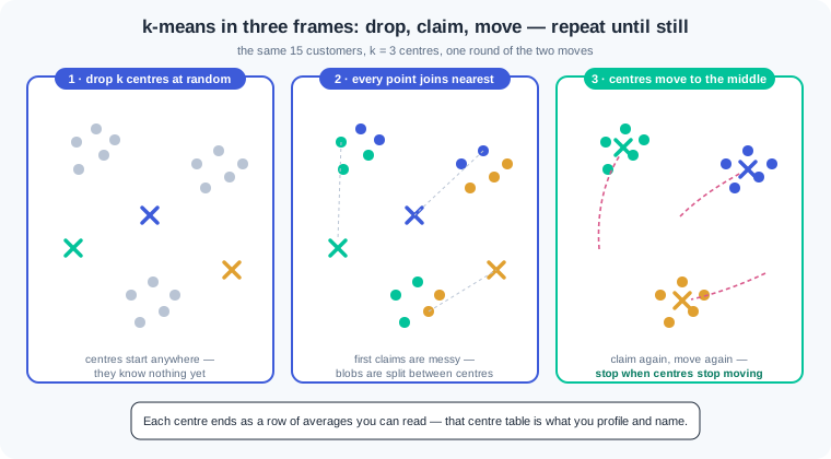
k-means — the workhorse clustering method: pick a number k, drop k centres into the feature space, and repeat two moves. Every point joins its nearest centre, then every centre moves to the middle of the points it claimed. The two moves repeat until the centres stop moving. The result is k tight groups, each described by its centre — a row of averages you can read.
Nothing in k-means tells you what k should be, so you gather evidence. The elbow method plots inertia — total squared distance from points to their centres — and looks for the bend where extra clusters stop paying. Silhouette score — a number from -1 to 1 that says how much closer each point sits to its own cluster than to the next one. Near 1 means clean, well-set groups; near 0, the split means little. Both are advice, not proof, and the final judge is whether the groups mean something to a human.
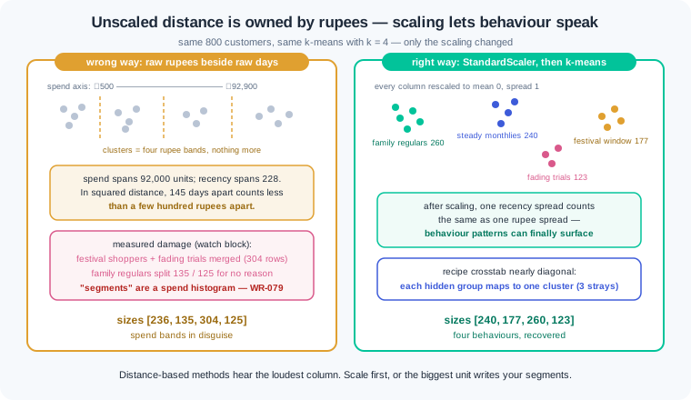
Before any distance is measured, scaling is mandatory, and the reason is the one 1.3 taught. Distance adds up squared differences, and a rupee column that spans 90,000 drowns a days column that spans 200. The wrong way: cluster raw rupee spend beside recency days, and every "segment" is a spend band in disguise. The right way: StandardScaler first, so each column speaks with equal volume, and real behaviour patterns can surface. WR-079 is a team that skipped this and presented salary bands as customer insight.
The second habit is naming, because k-means returns numbers, not meanings. "Cluster 3" tells a marketer nothing, and shipping bare cluster ids is how these projects die in review. Read each cluster's centre and compare it with the table averages. Then write the name the evidence supports: family regulars, festival-window shoppers, fading trials. A segment is a cluster plus a human-checked story plus an action.
Two more clustering tools earn a place in your kit. Hierarchical clustering merges the two closest rows, then the two closest groups, upward until one group remains. Dendrogram — the merge tree this builds, where cutting at any height gives you that many clusters. It answers "how does the data group at every zoom level" and needs no k up front; the cost is that it gets slow on large tables.
DBSCAN takes a different view: a cluster is any dense region, whatever its shape. You set a neighbourhood radius (eps) and a minimum crowd (min_samples), and DBSCAN grows clusters from dense cores. It never asks for k, it can trace curved shapes k-means cuts through, and it labels sparse points as noise (-1) instead of forcing them into a group. That noise label is a feature: the points no dense group wants are often the rows worth investigating.
Principal component analysis — a method that squeezes correlated columns into a few new axes called components. Each component is ranked by how much of the table's spread it keeps, and that share is its explained variance. Five correlated columns often fold into two components that keep most of the story. The prize is a 2D map of every customer, where distance means similarity — the same "similar things sit together" picture 3.4 draws for text embeddings. Train your eye here, where you can still read the rows behind every dot.
Anomaly detection — finding the rows unlike all others, without any example of "bad" to learn from. IsolationForest does it with random cuts: it grows trees that split the data at random, and rows that get isolated in very few cuts are the loners. Banks screen UPI transactions this way, and factories screen sensor readings for defects. The score ranks weirdness; the contamination setting decides how many rows get flagged, and WR-081 shows why that number must match your review capacity.
The honest limits close the module. With no target there is no accuracy, no recall, no sealed test — nothing from 1.5 applies directly. Evaluation becomes judgement: the silhouette score, stability across reruns, and whether a named segment changes a real decision. That bar is lower than a supervised scorecard, and pretending otherwise is how these projects overclaim. Say what the evidence supports, show the reruns, and let the segments earn their keep in a campaign.
Work inside ai-lab. One seeded world for the whole walkthrough: Varun's kirana-delivery customers, built from four hidden behaviour recipes so every claim below can be checked against the truth.
Build the customer table. Four recipes — A big families, B steady monthlies, C festival-window shoppers, D fading trials — with a recipe column we keep only to audit ourselves. Varun's real table would not have it:
import numpy as np
import pandas as pd

pd.set_option("display.width", 120)
pd.set_option("display.max_columns", 12)
rng = np.random.default_rng(42)

def group(name, n, rec, orders, spend):
    return pd.DataFrame({
        "recipe": name,
        "recency_days": rng.normal(rec[0], rec[1], n),
        "orders_12m": rng.normal(orders[0], orders[1], n),
        "spend_12m": rng.normal(spend[0], spend[1], n),
    })

customers = pd.concat([
    group("A", 260, (12, 5), (30, 4), (70000, 9000)),
    group("B", 240, (32, 8), (13, 2.2), (30000, 4500)),
    group("C", 180, (165, 22), (4, 1.2), (12000, 3000)),
    group("D", 120, (70, 12), (2, 0.8), (2400, 700)),
], ignore_index=True)
customers["recency_days"] = customers["recency_days"].clip(1).round()
customers["orders_12m"] = customers["orders_12m"].clip(1).round()
customers["spend_12m"] = customers["spend_12m"].clip(500).round(-1)
customers["app_sessions_12m"] = (customers["orders_12m"] * 3
                                 + rng.normal(0, 4, 800)).clip(1).round()
customers["months_active_12m"] = (customers["orders_12m"] * 0.45
                                  + rng.normal(0, 1, 800)).clip(1, 12).round()
feats = ["recency_days", "orders_12m", "spend_12m",
         "app_sessions_12m", "months_active_12m"]
print("customers:", len(customers))
print(customers[feats].describe().round(0).loc[["mean", "min", "50%", "max"]])
Output: customers: 800, then a summary where spend_12m runs from 500 to 92,940 while recency_days runs 1 to 229. Note the scales: rupees live in the tens of thousands, days and orders in the tens. That gap is about to matter. Note also that app_sessions_12m and months_active_12m were built from orders_12m — three columns carrying overlapping information, which is exactly what PCA will compress later.
The wrong way, measured: unscaled versus scaled. Same k-means, same k=4, run twice — once on raw columns, once after StandardScaler. The recipe crosstab is our answer sheet:
from sklearn.cluster import KMeans
from sklearn.preprocessing import StandardScaler

raw_km = KMeans(n_clusters=4, random_state=42, n_init=10).fit(customers[feats])
customers["raw_cluster"] = raw_km.labels_
print("unscaled sizes:", np.bincount(raw_km.labels_))
print(customers.groupby("raw_cluster")["spend_12m"].agg(["min", "max"]).round(-2))
print(pd.crosstab(customers["recipe"], customers["raw_cluster"]))

X = StandardScaler().fit_transform(customers[feats])
km = KMeans(n_clusters=4, random_state=42, n_init=10).fit(X)
customers["cluster"] = km.labels_
print("scaled sizes  :", np.bincount(km.labels_))
print(pd.crosstab(customers["recipe"], customers["cluster"]))
The unscaled run prints sizes [236 135 304 125], and the spend min/max table is the confession: cluster 2 spans ₹500–18,800, cluster 0 spans ₹19,800–42,200, cluster 3 spans ₹46,900–68,700, cluster 1 spans ₹69,100–92,900. Four non-overlapping rupee bands — the "segments" are a spend histogram. The crosstab shows the damage: recipe A is split 135/125 across two clusters for no behavioural reason, while C and D (festival shoppers and fading trials, 145 days of recency apart) are merged into one 304-row cluster, because a few hundred rupees apart is "identical" when distance only hears rupees. The scaled run prints sizes [240 177 260 123] and a nearly diagonal crosstab: A→260, B→240, C→177, D→120, with only 3 C rows sitting with D. Same algorithm, same data — the only change was giving every column an equal voice.
Choosing k: elbow plus silhouette. We pretend not to know there are four recipes, and ask the evidence:
from sklearn.metrics import silhouette_score

for k in range(2, 9):
    m = KMeans(n_clusters=k, random_state=42, n_init=10).fit(X)
    s = silhouette_score(X, m.labels_)
    print(f"k={k}   inertia: {m.inertia_:6.0f}   silhouette: {s:.2f}")
Output, one line per k: inertia falls 1136 → 391 → 206 → 167 → 146 → 132 → 116, while silhouette reads 0.64, 0.67, 0.70, 0.57, 0.45, 0.43, 0.37. Read the two witnesses together. Inertia always falls as k grows — more centres always sit closer — so you look for the bend: the drop from k=3 to k=4 (391 to 206) is the last big saving, and after that the curve flattens. The silhouette peaks at 0.70 for k=4 and then falls off a cliff to 0.57. Both witnesses point at 4, and the hidden recipes confirm they are right. When the two disagree, or the silhouette is flat across several k, that flatness is information too: the groups are not strongly separated, and WR-080 shows what happens when a team ships a k no evidence supports.
Profile and name the segments. Cluster ids are not deliverables. The centre table in original units is, once each row gets a name a marketer can act on:
profile = customers.groupby("cluster")[feats].mean().round(0)
profile.insert(0, "size", customers["cluster"].value_counts().sort_index())
names = {0: "Steady monthlies", 1: "Festival-window shoppers",
         2: "Family regulars", 3: "Fading trials"}
profile.index = [names[i] for i in profile.index]
print(profile)
The printed table is the lesson's key artefact. Family regulars: 260 customers, 12 days since last order, 30 orders, ₹69,338 a year, in the app weekly, active all 12 months — protect them. Steady monthlies: 240 customers, 13 orders, ₹30,038, active 6 months — grow their basket. Festival-window shoppers: 177 customers, 163 days quiet, 4 orders, ₹11,476, active 2 months — reach them before the next festival, not after. Fading trials: 123 customers, 2 orders, ₹2,732, one active month — a cheap win-back nudge or a conscious goodbye. Every name is an argument from the numbers beside it, and that is what separates a segment from a cluster id.
PCA: the whole table as one picture. Five scaled columns, several of them correlated, compressed to two components:
from sklearn.decomposition import PCA

pca = PCA(n_components=2).fit(X)
print("explained variance:", pca.explained_variance_ratio_.round(2),
      "  total:", pca.explained_variance_ratio_.sum().round(2))
pts = pca.transform(X)
customers[["pc1", "pc2"]] = pts.round(2)
print(customers.groupby("cluster")[["pc1", "pc2"]].mean().round(1))

xs = np.interp(pts[:, 0], (pts[:, 0].min(), pts[:, 0].max()), (0, 43)).astype(int)
ys = np.interp(pts[:, 1], (pts[:, 1].min(), pts[:, 1].max()), (11, 0)).astype(int)
grid = np.full((12, 44), " ", dtype=object)
for x, y, c in zip(xs, ys, customers["cluster"]):
    grid[y, x] = str(c)
print("\n".join("".join(r) for r in grid))
Output: explained variance: [0.9 0.08] total: 0.98 — the first component alone carries 90 percent of the variance, because orders, sessions and months-active all move together, and PCA folds that shared story into one axis. Two components keep 98 percent of five columns' information. The character grid then renders the map in plain text: the 2s (family regulars) form an island on the right, the 0s (steady monthlies) sit mid-left, and the 1s and 3s (festival shoppers, fading trials) occupy the low-engagement west with a visible gap between them. This is the picture to remember for 3.4: an embedding map of documents is this same plot, with the axes learned by a neural network instead of PCA — similar things sit together, and distance is meaning.
IsolationForest: the weirdest customers, ranked. Three ops tickets arrive — support suspects odd accounts. Append them and ask the forest for anomaly scores (lower = stranger):
from sklearn.ensemble import IsolationForest

tickets = pd.DataFrame({
    "recency_days": [3, 9, 420],
    "orders_12m": [58, 21, 1],
    "spend_12m": [1900, 940000, 800],
    "app_sessions_12m": [180, 66, 2],
    "months_active_12m": [12, 8, 1],
})
world = pd.concat([customers[feats], tickets], ignore_index=True)

iso = IsolationForest(contamination=0.01, random_state=42).fit(world)
world["anomaly_score"] = iso.score_samples(world[feats]).round(3)
print(world.nsmallest(8, "anomaly_score"))
The top of the list is exactly the three tickets. Rank one, score -0.702: 58 orders but only ₹1,900 in a year — order-and-refund behaviour, worth a fraud look. Rank two, -0.655: ₹9,40,000 across 21 orders — either a bulk reseller or a paise-versus-rupee data error, and either way not a "customer segment". Rank three, -0.630: 420 days of recency in a 12-month table — an impossible value, so a pipeline bug, not a person. The next five rows are honest extremes: the heaviest family regular (40 orders, score -0.607) and the quietest festival shoppers (about 190 days, near -0.60). That mix is normal and it is why every flag needs triage — data error, genuinely unusual, or explainable extreme — before anyone shouts fraud. The forest ranks; humans judge.
Work inside ai-lab. Every world is seeded: where a check states a number, your number must match it exactly.
If your numbers are close but not identical, triage in a fixed order before touching your code. Everything off by a little — every value drifting in the last decimal or two — points at a library version: run pip show scikit-learn, compare it with the pinned install line from 1.2, and match the pin, because the printed numbers were produced on that version. One number wildly off while the rest agree points at stale state: restart from a fresh kernel or a fresh python and run the file top to bottom, since seeded draws only reproduce when they happen in the same order from a clean start. Only when both checks pass and the numbers still disagree should you suspect your own logic — diff your script line by line against the printed code.
The segmentation project, end to end. An ethnic-wear e-commerce store wants segments it can act on, and you own the whole path from raw table to memo. In segments.py, with np.random.default_rng(7), build five hidden groups using the watch block's group() helper (columns drawn in the order recency, orders, spend inside each group), concatenated in this exact order: 150 rows ("P", (8,4), (24,4), (120000,15000)); 300 rows ("V", (30,9), (11,2.5), (33000,6000)); 250 rows ("S", (95,18), (5,1.5), (15000,4000)); 180 rows ("N", (12,6), (2,0.8), (4200,1200)); 120 rows ("Z", (260,35), (1,0.5), (2000,700)). Clip and round exactly as the watch block does (recency and orders .clip(1).round(), spend .clip(500).round(-1)). Features are the three RFM columns only. Now work as if the recipe column did not exist: scale with StandardScaler, print inertia and silhouette for k=2 through 9, pick k with a one-line defence, fit the final model with random_state=42, n_init=10, print sizes and the centre table in original units, name every segment, and audit yourself with the recipe crosstab at the end. Close with a memo: for each segment, five lines — who they are, the two numbers that prove it, one campaign action, one risk if ignored, one metric to watch next quarter. Check: 1000 rows; the elbow alone is ambiguous but the silhouette settles it — 0.66 at k=3, a dip to 0.59 at k=4, a clear peak of 0.69 at k=5, and nothing better after; your final sizes print [298 120 150 249 183]; the centre table shows a 150-customer premium segment at 7 days recency, 24 orders, ₹1,19,265 and a 120-customer dormant segment at 259 days, 1 order, ₹1,934; the crosstab confirms every recipe maps to one cluster with at most 4 strays; your memo has five named segments and five lines each, and no segment is named "Cluster 0".
Anomaly triage, the ops-queue way. Your review team can inspect 20 accounts, not 200, and each flag needs a verdict. In triage.py, with np.random.default_rng(11), build a base of three groups using the same group() helper and clipping, concatenated in this order: 900 rows ("regular", (25,10), (12,3), (30000,6000)); 350 rows ("loyal", (10,5), (28,5), (72000,10000)); 250 rows ("occasional", (120,30), (4,1.5), (12000,3500)). Then append, unclipped and in this exact order, nine seeded oddities with recipe "odd" — recency [999, 500, 12, 21, 15, 2, 4, 1, 3], orders [6, 9, 14, 0, 14, 45, 38, 9, 1], spend [21000, 27000, 2850000, 15000, 60, 3600, 260000, 180000, 150000]. Fit IsolationForest(contamination=0.013, random_state=42) on the three feature columns, print the 20 lowest score_samples rows, and verify the flag count equals your team's capacity. Build a triage table: for each of the 20, one verdict — data-error (value impossible for a 12-month table), genuinely-unusual (possible but suspicious behaviour), or explainable (an honest extreme of a known group) — plus a one-line reason. Finish with three sentences on the rows the forest missed and what cheap rule-based checks you would add beside it. Check: 1509 rows and exactly 20 flags; the top-20 catches 7 of the 9 seeded oddities, led by the 999-day sentinel at score -0.715 and the 45-order refund pattern at -0.700; your verdicts sort the top-20 into 3 data-errors (999 days, 500 days, ₹28,50,000), 4 genuinely-unusual (45 orders/₹3,600, 38 orders/₹2,60,000, 9 orders/₹1,80,000, 1 order/₹1,50,000) and 13 explainable extremes; your closing sentences name the two misses — 0 orders with ₹15,000, and ₹60 across 14 orders — explain that neither has a single extreme feature so isolation cuts find them slowly, and propose rule checks such as spend-per-order bounds and impossible-value guards.
Shapes k-means cannot cut, and the noise DBSCAN refuses to force. In shapes.py, build two interleaved crescents with make_moons(n_samples=600, noise=0.07, random_state=42), then append 40 scatter points drawn with np.random.default_rng(3) — x uniform in (-1.5, 2.5), y uniform in (-1.0, 1.5) — keeping a truth array where the crescents are 0 and 1 and the scatter is -1. Part (a): fit KMeans(n_clusters=2, random_state=42, n_init=10) and print the truth-versus-label crosstab. Part (b): fit DBSCAN(min_samples=8) for eps 0.1, 0.2 and 0.3, printing cluster count and noise count for each, then the crosstab for eps=0.2. Part (c): a three-line memo — one line on why k-means fails here, one on what the -1 label means and why deleting those rows is wrong, one naming a real table where you would reach for DBSCAN first. Check: 640 points; the k-means crosstab shows both crescents split — one cluster holds 219 of crescent 0 plus 74 of crescent 1, the other holds 81 plus 226 — so 155 crescent points sit with the wrong crowd; the eps sweep prints 2 clusters/47 noise at 0.1, 2 clusters/19 noise at 0.2, and 1 cluster/17 noise at 0.3 (one radius merges the crescents); at eps=0.2 the crosstab is perfect — 300 and 300 with zero mixing — and 19 of the 40 scatter points are labelled -1 while 21 landed dense enough to be absorbed; your memo says k-means assumes round blobs around centres, noise points are review candidates rather than bad data, and your example names something shaped or density-based, like delivery GPS traces or fraud bursts.
The unsupervised review checklist you will keep. Write segmentation_review.md, the one-page audit you will run on every clustering or anomaly project, including your own. Five sections, each with at least two questions in your own words: scaling (would the clusters survive a unit change — rupees to paise?), choosing k (what evidence, and was stability across reruns checked?), naming (does every segment have a name argued from its centre, with an action?), honest limits (what claim is being made without a target, and what would falsify it?), and anomaly flags (does the flag rate match review capacity, and who triages?). End with a verdict drill — three proposals land on your desk: (i) "we clustered raw incomes and got five sharp customer segments", (ii) "k=5, same as the blog post our senior shared", (iii) "we set contamination to 0.10 so we never miss a fraud". Under each, write the failure you expect, the checklist question that catches it, and the linked War Room id. Check: five sections and at least ten questions; the verdicts predict income-band segments for (i), unstable meaningless clusters for (ii), and an unreviewable flood of flags for (iii); they cite WR-079, WR-080 and WR-081 in that order; at least one question asks whether the segments survive a rerun with a different seed, and at least one asks what business decision changes if the segments are real.
Three unsupervised disasters cover most of what this lesson meets in production. Each has a War Room entry with the full diagnosis path:
- WR-079 — the segments that were salary bands. An unscaled income column owned every distance, so four "behavioural segments" were four income bands wearing costumes; scaling first and auditing what drives each cluster is the fix and the habit.
- WR-080 — the k nobody questioned. A k copied from a blog post shipped segments that reshuffled on every rerun and meant nothing to marketing; elbow plus silhouette plus a stability check plus a business read is the evidence a k must carry.
- WR-081 — the anomaly flood. A contamination setting chosen for "safety" flagged thousands a week, the queue was ignored within a month, and a real fraud sailed through unread; sizing the flag rate to review capacity with triage tiers is the way back.
Unsupervised learning finds structure in tables that have no answer column: groups, shapes, odd rows and compressed views. k-means claims points and moves centres until they settle, and it needs scaled features because raw rupees own any unscaled distance. Pick k with the elbow and the silhouette score together, then check the groups survive a rerun. Ship named segments argued from their centres, never bare ids, and let PCA draw the whole table as one two-axis picture. There is no accuracy without a target, so judge clusters by their spread, their stability and their business use, and say that limit out loud.
- Indian banks and UPI apps screen payment streams for odd transactions. Scores rank the strangeness, and a queue sized to the review team goes to humans — the triage drill from exercise 2.
- Quick-commerce and e-commerce teams rebuild customer segments every quarter. The deck that survives review carries named segments with evidence, not a cluster id column.
- GenAI retrieval maps in 3.4 rest on the same geometry: similar documents sit together. You learn to read that picture here first, on rows you can still open and check.
Answer these before opening the gate assessment. Each question names its type.
type=output-prediction— A teammate runs k-means with k=4 on raw columns wherespend_12mspans ₹500 to ₹92,000 andrecency_daysspans 1 to 229. Predict what organises the four clusters, what the per-cluster spend min/max table will look like, and which two genuinely different behaviour groups are most likely to be merged. Then predict what changes after StandardScaler.type=debug— A segmentation notebook produces different segments every run, and marketing has stopped trusting the deck. You find: norandom_state,n_init=1, raw unscaled features, and k=7 taken from a tutorial. Order these four faults by how much damage each does to stability and meaning, and give the two-line fix.type=interpretation— A centre table reads: segment A — 11 days recency, 28 orders, ₹65,000; segment B — 160 days, 4 orders, ₹12,500; segment C — 70 days, 2 orders, ₹2,600. Name each segment from the evidence, pick the one segment for a pre-Diwali win-back budget, and say which number you would watch to know the campaign worked.type=scenario-judgement— A fraud lead wantscontamination=0.08on 12,000 daily transactions "so nothing slips through", while the review team can inspect 30 cases a day. Judge the proposal with the arithmetic, name what happens to the queue and to trust in the flags, and state the version you would approve.type=trade-off— For grouping delivery locations across a city, compare k-means, DBSCAN and hierarchical clustering. Give one concrete strength and one concrete cost of each, and say which you would try first when zones are odd-shaped and some addresses are one-off deliveries.
Explain to a friend who runs a kirana shop how you would organise a truckload of unlabelled new stock: you group similar items onto shelves (clustering), you decide how many shelves by seeing when adding one more stops helping (choosing k), you name each shelf only after looking at what landed on it (naming segments), and the odd item that fits no shelf goes to the counter for a closer look (anomaly detection). Use at most 4 sentences and no word fancier than "shelf". If your friend can say why the shelf names come last, not first, you own this module.