Feature engineering & encoding
Monday morning in Ludhiana. Deepak's churn model at a grocery-delivery startup catches almost no one, and his fix list says: try a bigger model. His mentor disagrees. She opens the raw table and points at three sleeping columns — income, order dates, city. The model cannot read a date, she says, and it has never heard of a ratio. Build the columns it can read. By evening, the same plain model catches twenty-seven churners instead of zero.
- Better features beat fancier models on business tables, and this lesson proves it with scores you can re-run — interview panels probe exactly this.
- "How would you handle 3,000 pincodes?" — that one encoding question screens freshers at many Indian fintech and banking teams.
- The Pipeline habit you build today is what makes a model fit to ship, and the serving work in Phase 4 assumes you have it.
Module 1.4 crowned boosted trees for tables, and this lesson adds the deeper truth. On tabular data, the biggest wins come from the columns, not the model. Feature engineering — reshaping raw columns into signals a model can read. In the demo below, a plain logistic model with three built columns beats a boosted model on raw columns by twenty points. A model can only see what your columns show it.
Three numeric moves cover most tabular wins. A ratio divides two columns to expose a relationship — EMI over income says "stretched" in one number, where neither column alone does. A difference turns two values into a gap, like days-since-last-order from an order date. A log transform tames skewed rupee amounts, so a few crore earners stop drowning out ordinary salaries.
A raw date is unreadable to a model, yet it hides several honest features. Day-of-week separates weekend family orders from office-lunch orders. Day-of-month captures India's salary cycle — orders surge in the first week, and EMI payments bounce at month-end. A festival flag marks Diwali or Eid weeks, when every pattern shifts. One timestamp column can feed half a dozen features.
Words need work too, because models eat only numbers. One-hot encoding — one new column per category, holding 1 where the row matches. It is the honest default for a handful of values, like five cities. Ordinal encoding gives each value a rank number, and it is right only when the order is real, like school then graduate then postgraduate. Numbering cities A to Z invents a fake order, and the model will trust it.
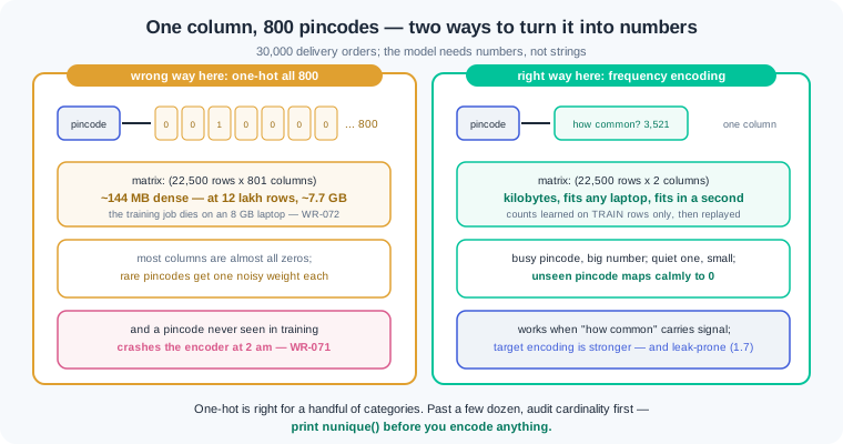
One-hot has a failure mode, and its name is cardinality. A pincode column with 800 values becomes 800 columns, because the matrix grows as rows times categories. Frequency encoding — replacing each category with how often it appears in the training data — keeps one column and often loses nothing. Target encoding — replacing each category with the average target value seen for it — is stronger still, and it is the most leak-prone tool in this phase. Treat it with care until module 1.7 teaches the full leakage drill.
Three quiet families finish the toolkit. Text-lite features read a message column without any language model: the message length, or a flag for a keyword like "refund". Binning folds a numeric column into a few labelled ranges, useful when a relationship bends instead of sloping. A missing-value indicator — a 0/1 column marking where a value was absent — earns its place because a blank is often a clue. At an NBFC, a missing income field says something about the person who applied.
Now the discipline that carries all of it. The wrong way: transform the DataFrame by hand in the training notebook, then rewrite those steps inside the scoring script. Every learned number — the scaler's mean, the encoder's city list, the frequency counts — drifts between the two copies, and predictions go silently wrong. The right way: build the steps once inside a Pipeline, fit on training rows only, and let predict replay identical learned numbers on every future row.
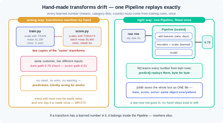
ColumnTransformer — the sklearn piece that routes each column group to its own transform: the city column to an encoder, the numeric columns to a scaler. Wrapped in a Pipeline with the model, the whole path becomes one object speaking fit and predict, the two verbs from 1.2. joblib saves that object as one file, and the scoring side loads it and calls predict on a raw row. Hand-transforming DataFrames at predict time is not a style choice; in this course it is the wrong way, full stop.
Work inside ai-lab. The churn world moves to Deepak's company in Ludhiana and gains the richer raw table real teams inherit: a city, an income, and a proper order date.
The before picture — good columns, asleep. Seeded world, split, and a logistic model on the raw numeric columns only (the model cannot eat the date or the city yet):
import numpy as np
import pandas as pd
from sklearn.linear_model import LogisticRegression
from sklearn.model_selection import train_test_split
from sklearn.pipeline import make_pipeline
from sklearn.preprocessing import StandardScaler
from sklearn.metrics import recall_score

rng = np.random.default_rng(42)
n = 500
snapshot = pd.Timestamp("2026-06-30")
customers = pd.DataFrame({
    "city": rng.choice(["Ludhiana", "Jalandhar", "Amritsar",
                        "Patiala", "Bathinda"], size=n),
    "monthly_income": rng.integers(18000, 120000, size=n),
    "orders_last_90d": rng.poisson(6, size=n),
    "avg_order_value": rng.integers(120, 900, size=n),
})
customers["last_order_date"] = snapshot - pd.to_timedelta(
    rng.integers(1, 120, size=n), unit="D")

spend_share = (customers["avg_order_value"]
               * customers["orders_last_90d"] / 3) / customers["monthly_income"]
days_since = (snapshot - customers["last_order_date"]).dt.days
salary_week = (customers["last_order_date"].dt.day <= 7).astype(int)
risk = (-3.0 + 0.05 * days_since - 25 * spend_share
        - 1.3 * salary_week - 0.15 * customers["orders_last_90d"])
customers["churned"] = (rng.random(n) < 1 / (1 + np.exp(-risk))).astype(int)

raw_feats = ["monthly_income", "orders_last_90d", "avg_order_value"]
X_train, X_test, y_train, y_test = train_test_split(
    customers.drop(columns="churned"), customers["churned"],
    test_size=0.25, random_state=42, stratify=customers["churned"])

before = make_pipeline(StandardScaler(), LogisticRegression(max_iter=1000))
before.fit(X_train[raw_feats], y_train)
bp = before.predict(X_test[raw_feats])
print("churn rate:", round(customers["churned"].mean(), 2))
print(f"raw columns   accuracy: {before.score(X_test[raw_feats], y_test):.2f}"
      f"   recall: {recall_score(y_test, bp):.2f}"
      f"   caught: {((bp == 1) & (y_test == 1)).sum()} of {y_test.sum()}")
churn rate: 0.31
raw columns   accuracy: 0.69   recall: 0.00   caught: 0 of 39
Read it honestly, 1.5 style. Accuracy 0.69 equals the do-nothing baseline (69 percent of test customers stayed), and recall 0.00 means the model catches nobody. The generation formula upstairs shows why: churn lives in days-since-order, in spend as a share of income, and in a salary-week habit — none of which is a column the model received. The information exists in the raw table; it is written in a language the model cannot read.
Three engineered columns wake the table up. One feature function builds a difference, a ratio, and a calendar flag; then the same plain model gets a rematch — and a boosted model on raw columns joins, to settle 1.4's question:
def add_features(df):
    out = df.copy()
    out["days_since_last_order"] = (snapshot - out["last_order_date"]).dt.days
    out["spend_share"] = (out["avg_order_value"]
                          * out["orders_last_90d"] / 3) / out["monthly_income"]
    out["salary_week_order"] = (out["last_order_date"].dt.day <= 7).astype(int)
    return out

eng_feats = raw_feats + ["days_since_last_order",
                         "spend_share", "salary_week_order"]
after = make_pipeline(StandardScaler(), LogisticRegression(max_iter=1000))
after.fit(add_features(X_train)[eng_feats], y_train)
ap = after.predict(add_features(X_test)[eng_feats])
print(f"engineered    accuracy: "
      f"{after.score(add_features(X_test)[eng_feats], y_test):.2f}"
      f"   recall: {recall_score(y_test, ap):.2f}"
      f"   caught: {((ap == 1) & (y_test == 1)).sum()} of {y_test.sum()}")

from sklearn.ensemble import HistGradientBoostingClassifier
hgb = HistGradientBoostingClassifier(random_state=42)
hgb.fit(X_train[raw_feats], y_train)
hp = hgb.predict(X_test[raw_feats])
print(f"boosted, raw  accuracy: {hgb.score(X_test[raw_feats], y_test):.2f}"
      f"   recall: {recall_score(y_test, hp):.2f}"
      f"   caught: {((hp == 1) & (y_test == 1)).sum()} of {y_test.sum()}")
Output: engineered accuracy: 0.83 recall: 0.69 caught: 27 of 39, then boosted, raw accuracy: 0.63 recall: 0.23 caught: 9 of 39. Same model, same split — three new columns moved accuracy from 0.69 to 0.83 and the catch count from 0 to 27. Meanwhile 1.4's champion, gradient boosting, scores 0.63 on the raw columns: twenty points behind a plain logistic model that was handed a ratio, a difference and a calendar flag. That is the lesson's headline, measured: the win was in the features. days_since_last_order is a difference of dates, spend_share is a ratio (roughly monthly spend over income), and salary_week_order reads the salary cycle off last_order_date.dt.day.
Encoding the city — and the trap waiting at 800. ColumnTransformer routes each column group to its own transform; then a bigger table shows what happens when the category count explodes, and what frequency encoding saves:
from sklearn.compose import ColumnTransformer
from sklearn.preprocessing import OneHotEncoder

small = ColumnTransformer([
    ("city", OneHotEncoder(handle_unknown="ignore"), ["city"]),
    ("num", StandardScaler(), raw_feats),
])
out = small.fit_transform(X_train)
print("5 cities, one-hot:", out.shape)
print(small.get_feature_names_out()[:5])

rng2 = np.random.default_rng(7)
orders = pd.DataFrame({
    "pincode": rng2.choice([str(p) for p in range(140001, 140901)], size=20000)})
wide = OneHotEncoder(sparse_output=False).fit_transform(orders)
print("900 pincodes, one-hot:", wide.shape,
      f"  ~{wide.nbytes / 1e6:.0f} MB dense")

counts = orders["pincode"].value_counts()
orders["pincode_freq"] = orders["pincode"].map(counts)
print("frequency encoded  :", orders[["pincode_freq"]].shape,
      "  sample:", orders["pincode_freq"].head(3).tolist())
Output, four prints: 5 cities, one-hot: (375, 8), then the first five column names — city__city_Amritsar, city__city_Bathinda, city__city_Jalandhar, city__city_Ludhiana, city__city_Patiala — then 900 pincodes, one-hot: (20000, 900) ~144 MB dense, then frequency encoded : (20000, 1) sample: [35, 23, 14]. The small case is healthy: five cities plus three scaled numerics gives eight tidy columns. The big case is the trap: 900 Punjab-style pincodes became 900 columns and 144 MB for a mere 20,000 rows — at 12 lakh rows the same arithmetic passes 8 GB, and the training job dies (WR-072). Frequency encoding answers with one column: this pincode appeared 35 times, that one 23. Note handle_unknown="ignore" on the city encoder — the quiet setting that keeps 2 am pages away (WR-071).
Seal everything into one Pipeline. Feature function, encoders, scaler and model become a single fitted object; joblib ships it; a raw row — date, city, rupees — goes straight in:
import joblib
from sklearn.pipeline import Pipeline
from sklearn.preprocessing import FunctionTransformer

churn_pipe = Pipeline([
    ("features", FunctionTransformer(add_features)),
    ("prep", ColumnTransformer([
        ("city", OneHotEncoder(handle_unknown="ignore"), ["city"]),
        ("num", StandardScaler(), eng_feats),
    ])),
    ("model", LogisticRegression(max_iter=1000)),
])
churn_pipe.fit(X_train, y_train)
pp = churn_pipe.predict(X_test)
print(f"pipeline      accuracy: {churn_pipe.score(X_test, y_test):.2f}"
      f"   recall: {recall_score(y_test, pp):.2f}")

joblib.dump(churn_pipe, "churn_pipeline.joblib")
loaded = joblib.load("churn_pipeline.joblib")

new_customer = pd.DataFrame([{
    "city": "Jalandhar",
    "monthly_income": 32000,
    "orders_last_90d": 2,
    "avg_order_value": 250,
    "last_order_date": pd.Timestamp("2026-04-12"),
}])
print("prediction :", loaded.predict(new_customer)[0])
print("churn prob :", loaded.predict_proba(new_customer)[0, 1].round(2))
pipeline      accuracy: 0.82   recall: 0.67
prediction : 1
churn prob : 0.7
Walk the sealed box top to bottom. fit ran once, on training rows only: the feature step derived the engineered columns, the encoder memorised five cities, the scaler memorised training means, the model learned its weights. predict then replayed those exact learned numbers on the test set (0.82, within noise of the hand-built 0.83) and on a completely raw new customer — a Jalandhar account, silent since 12 April, ordering mid-month. No hand transform exists at predict time, so no hand transform can drift (WR-070). One file, churn_pipeline.joblib, now carries the entire path from raw row to verdict — this is the object your Phase 4 API will serve.
Work inside ai-lab. Every world is seeded: where a check states a number, your number must match it exactly.
If your numbers are close but not identical, triage in a fixed order before touching your code. Everything off by a little — every value drifting in the last decimal or two — points at a library version: run pip show scikit-learn, compare it with the pinned install line from 1.2, and match the pin, because the printed numbers were produced on that version. One number wildly off while the rest agree points at stale state: restart from a fresh kernel or a fresh python and run the file top to bottom, since seeded draws only reproduce when they happen in the same order from a clean start. Only when both checks pass and the numbers still disagree should you suspect your own logic — diff your script line by line against the printed code.
The feature hunt, on loans. An NBFC world with hidden ratios. Build it in feature_hunt.py with np.random.default_rng(21), 600 rows, columns drawn in this exact order: monthly_income integers 25,000–150,000; emi integers 2,000–40,000; months_on_book integers 3–48; bounced_payments Poisson(mean 1.0). Then defaulted = 1 with probability sigmoid(-4.8 + 9*(emi/monthly_income) + 15*(bounced_payments/months_on_book)), drawn with one rng.random(600) call. Split test_size 0.25, random_state=42, stratified. Fix the model once and never touch it: make_pipeline(StandardScaler(), LogisticRegression(max_iter=1000, class_weight="balanced")). Before running anything, write five candidate features as comments — emi_ratio (emi over income), bounce_rate (bounces over months), plus three inventions of your own (try income_left, log_income, emi_x_months). Score the 4 raw columns, then each candidate added alone, keeping a candidate only if it raises defaulters-caught by at least 2. Fit a final model on raw plus the keepers and print one honest table: feature set, accuracy, recall, caught-of-40 — failures included. Check: the raw row prints accuracy 0.88 and 28 of 40 caught; emi_ratio alone lifts the catch to 30 and bounce_rate alone to 32, so both are kept; income_left and emi_x_months add zero and log_income adds one, so all three are dropped; the final row prints accuracy 0.91, recall 0.80, 32 of 40 caught; your table still shows the three failed candidates with their unmoved scores.
Port 1.2's loose script into one Pipeline. In 1.2 you trained churn models with hand-picked columns, and the city column sat out. Rebuild that world exactly in pipeline_port.py: seed 42, n=400, columns drawn city first (Patna, Gaya, Muzaffarpur), then orders_last_90d Poisson(6), days_since_last_order integers 1–120, avg_order_value integers 120–900, churn from risk = -3.0 + 0.07*days_since_last_order - 0.5*orders_last_90d. Same split as always (0.25, seed 42, stratified). Now build ONE Pipeline: a ColumnTransformer sending city to OneHotEncoder(handle_unknown="ignore") and the three numerics to StandardScaler, then LogisticRegression(max_iter=1000, class_weight="balanced"). Exactly one fit call in the whole script. Print accuracy, recall and caught-of-26; dump the fitted pipeline with joblib; then, in a separate score_one.py that imports nothing from the training script, load the file and predict the raw row {city: "Gaya", orders_last_90d: 1, days_since_last_order: 95, avg_order_value: 260}. Close with two written sentences comparing your scores against 1.2's city-less balanced model (0.84 accuracy, 0.81 recall) and explaining what the city column contributed. Check: the pipeline prints accuracy 0.81, recall 0.73, 19 of 26 caught; score_one.py prints prediction 1 with probability 0.99 from the raw row, with no fit and no scaler code anywhere in it; your two sentences say the city added noise rather than signal — the churn formula never used it — so the score dipped slightly, and one-hot cannot invent information that is not there.
The pincode audit. A Bengaluru quick-commerce logistics table where busy pincodes run late. In pincode_audit.py, with np.random.default_rng(11): 30,000 orders; pincode drawn from the 800 strings 560001–560800 with weights proportional to 1/(rank+20) (rank 0–799, normalised), so a busy head and a long tail; distance_km uniform 1–15 rounded to 1 decimal. Compute each pincode's order count with value_counts, then late = 1 with probability sigmoid(-4.4 + 0.10*distance_km + 0.55*log1p(count)). Split 0.25, seed 42, stratified. Route A: a Pipeline one-hot encoding pincode (handle_unknown="ignore", sparse_output=False) beside scaled distance, into LogisticRegression(max_iter=1000, class_weight="balanced"); print the transformed training matrix's shape and megabytes, then accuracy and recall. Route B: frequency encoding — map each pincode to its count in the TRAINING split only, unseen maps to 0 — then scale and fit the same model; print shape and scores. Then the 2 am test: fit a default OneHotEncoder (no handle_unknown setting) on training pincodes and transform the unseen pincode 560999 inside try/except, printing the error's first line; show Route A and Route B both score that row calmly. Finish with a two-line memory note extrapolating the dense matrix to 12 lakh rows. Check: Route A prints shape (22500, 801) and about 144 MB, accuracy 0.60, recall 0.61; Route B prints shape (22500, 2), accuracy 0.63, recall 0.57 — one learned column keeping pace with 800; the caught exception mentions Found unknown categories; your memory note lands near 7.7 GB for 12 lakh rows and names the cardinality audit as the habit that prevents WR-072.
Silent signals: missingness and message text. A support-ticket churn table where the loudest signals hide in a blank field and a complaint message. In silent_signals.py, with np.random.default_rng(9), 800 tickets, draws in this order: months_active integers 1–36; orders_last_90d Poisson(5); asks_refund as rng.random(800) < 0.30; message words as rng.choice(pool, size=(800, 8)) with pool = ["app", "slow", "late", "order", "wrong", "item", "delivery", "money", "back", "help"], joined with spaces, prefixed with "refund " where asks_refund is true; linked as rng.random(800) < 0.60; monthly_income integers 18,000–90,000 as float, set to np.nan where not linked. Churn probability: sigmoid(-2.4 + 1.3*unlinked + 1.8*asks_refund + 0.02*(msg_len - msg_len.mean()) - 0.10*orders_last_90d) where msg_len is message character length. Split 0.25, seed 42, stratified. Build three pipelines with LogisticRegression(max_iter=1000, class_weight="balanced"), each imputing income with the median inside the pipeline: (A) the three numeric columns only; (B) same, with SimpleImputer(strategy="median", add_indicator=True) so a missing-value indicator column appears; (C) B plus two text-lite features built in a feature function — msg_length and an asks_refund keyword flag from str.contains("refund"). Print one table: version, accuracy, recall, caught-of-42, and below it three sentences naming what each addition contributed and why a blank income field carried signal. Check: A prints accuracy 0.49, recall 0.43, 18 of 42; B lifts the catch to 23; C prints accuracy 0.62, recall 0.67, 28 of 42; the income column is roughly 38 percent missing and no imputation happens outside the pipeline; your sentences connect the indicator's lift to unlinked accounts churning more, not to the imputed values themselves.
Three feature-engineering failures cover most of what this lesson meets in production. Each has a War Room entry with the full diagnosis path:
- WR-070 — the transforms that drifted. A scoring script re-implemented the training notebook's hand-made transforms with its own means and category lists; predictions went silently wrong for weeks — no crash, no log line. One fitted Pipeline, saved and loaded everywhere, plus a one-row parity test, is the fix.
- WR-071 — the city the encoder never saw. Production sent a category value the encoder was never fitted on, and the service died at 2 am with
Found unknown categories— the quieter variant encodes it as all zeros and tells nobody.handle_unknown="ignore"plus an unseen-category alert plus a retrain cadence fixes all three layers. - WR-072 — the one-hot that ate the training job. One-hotting 3,000 pincodes turned a modest table into gigabytes and the OS killed the job; rows times categories is the arithmetic nobody ran. A cardinality audit before encoding, sparse output, and frequency or grouped encodings are the way back.
On tables, the biggest wins come from building better columns, not from swapping in fancier models. Ratios, differences, log transforms, calendar flags and text-lite features turn raw columns into signals a model can read. One-hot suits a handful of values, ordinal fits only a real order, and frequency or target encoding handles the huge columns. Blanks carry signal too, so keep a missing-value indicator instead of filling them in silence. Every transform with a learned number lives inside one fitted Pipeline, learned on train rows only and replayed the same way on every new row.
- Bank and NBFC credit scorecards run on engineered ratios. The FOIR — fixed obligations to income ratio — that decides Indian loan approvals is the same EMI-over-income feature you built today.
- Quick-commerce and food-delivery firms feed churn and demand models calendar features first. Payday weeks, Diwali and Eid flags, and day-of-week curves add more lift than model swaps.
- UPI fraud engines lean on frequency-style features: how common is this device, this merchant, this hour for this user. Merchant ids run into lakhs of values, so one-hot is out of the question there.
Answer these before opening the gate assessment. Each question names its type.
type=output-prediction— AColumnTransformerone-hot encodes a 5-city column and scales 3 numeric columns, then is fitted on 375 training rows. Predict the transformed matrix's shape, and the shape if the city column instead held 900 distinct pincodes. State the memory implication of the second shape in one sentence.type=debug— At 2:04 am the scoring service throwsValueError: Found unknown categories ['Moga'] in column 0 during transform. Name the cause in one sentence, the one-line change that stops the crash, and the monitoring you would add because that change alone makes the failure silent.type=interpretation— A before/after table reads: raw columns 0.88 accuracy, 28 caught; +emi_ratio 30 caught; +bounce_rate 32 caught; +log_income 29 caught; +income_left 28 caught. The team wants to ship all five features "since more information cannot hurt". Read the table back to them: which features earned a place, which did not, and what does the honest report look like?type=scenario-judgement— A teammate's plan for the new delivery-delay model: one-hot all 3,000 pincodes, and copy the scaling code into the scoring script "to keep the service independent of sklearn". Judge both halves of the plan, with the failure each one produces and the alternative you would insist on.type=trade-off— For an 800-value merchant-category column, compare one-hot encoding, frequency encoding and target encoding. Give one concrete strength and one concrete cost of each, and name the one that must wait for module 1.7's leakage discipline before you are allowed to trust it.
Explain to a friend who cooks why a model fed raw columns is like a cook handed a locked spice box: the flavour exists, but nothing can reach it. Cover why you built the ratio and the days-since columns before touching a fancier model, and why the same recipe must season the dish identically at practice and at the wedding — your training and scoring paths. Use at most 4 sentences and no word fancier than "recipe". If your friend can say why the recipe is written down once and reused, not remembered twice, you own this module.