Trees, RF, boosting, XGBoost
Thursday afternoon in Vadodara. Vikram scores vehicle loans at an NBFC. His logistic model from the last module works, but a senior asks a hard question: why did it reject applicant 4127? Vikram reads coefficients aloud and watches eyes glaze. Then the branch manager rejects the same file in ten seconds. Is the EMI above a third of income? Is the account under six months old? Two questions, one decision. Build models that ask questions like her, his senior says. On tables, they win.
- Boosted trees win most tabular problems — churn, credit risk, fraud — the exact tables Indian companies hire freshers to work on.
- "Explain random forest" and "why did XGBoost beat your logistic model" are standard fresher interview questions.
- The whole tree family trains in seconds on an 8GB laptop, with no GPU and no scaling pipeline to maintain.
A decision tree — a model that learns a chain of if-else questions from data. Each question splits the rows into two groups, and each final group carries a verdict. The branch manager's two questions were a hand-made tree; ours will be learned from rows. Unlike the coefficients of 1.3, a fitted tree can be printed and read as plain rules. That makes it the most explainable model a bank auditor will ever meet.
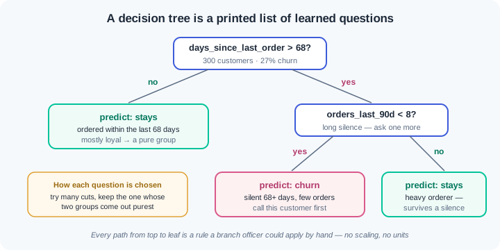
How does the tree pick its questions? At every step it tries many candidate cuts and measures each with impurity — a score of how mixed a group is. A group of all churners, or all loyal customers, is pure; a fifty-fifty group is fully mixed. The tree keeps the cut whose two children are purest, then repeats inside each child. You will even see it split when both children vote the same way, because one child became much purer — purity drives splits, not the final label.
Notice what every question looks at: is this value above a cut, yes or no. A cut cares about order, never about units, so trees need no feature scaling. The pipeline and the ConvergenceWarning battles of 1.3 do not exist here. Rupees, days and counts can sit side by side untouched. That is one quiet reason tree models are loved on messy business tables.
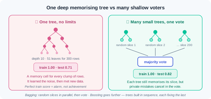
This freedom has a cost, and you have already met it. In 1.2 an unlimited tree scored a perfect train result and then 0.71 on the test set, because it memorised all 300 rows, noise included. The wrong way is trusting that one deep tree. The right way is a random forest, built by bagging — training many trees, each on a random slice of rows and features, then letting them vote. Each tree still memorises its own slice, but their private mistakes cancel in the vote, and the shared signal survives.
A forest's trees vote as equals and never talk to each other. There is a second, stronger recipe: boosting — training trees one after another, where each new tree focuses on the mistakes the earlier ones made. Gradient boosting is the version that measures those mistakes with a loss slope, the downhill idea from 0.7 again. In scikit-learn you get it as HistGradientBoostingClassifier, fast on a plain laptop with nothing new to install. XGBoost and LightGBM are the famous industry libraries built on the same idea — name them in interviews, and your sklearn knobs transfer almost one to one.
Tree models also hand you feature importance — a score for how much each feature helped the splits. It looks like a free explanation, and managers love the chart. Treat it as a lead, not a verdict. The default score splits credit between correlated features and inflates columns with many possible cut points, so a noise column can outrank a real one. The honest cross-check is permutation importance — shuffle one column on the test set and watch how far the score falls; module 1.11 goes deeper.
Why does this family rule tabular data? Business tables mix scales, hide sharp thresholds, and hold feature interactions, and trees cut along all of them without preprocessing. On such tables, boosted trees still beat neural networks in most benchmarks and most Indian production systems. They are the wrong tool when data is tiny, when a regulator must read the whole model, or when the input is images or text — deep learning owns those. Phase 2 starts there; today you take the crown for tables.
Work inside ai-lab. Everything below runs on the scikit-learn you installed in 1.2 — no new packages, and notice there is no scaler anywhere in this lesson.
Grow a small tree and read it aloud. Same seeded churn world as 1.2 (Aditya's company, same target), then a depth-2 tree, printed:
import numpy as np
import pandas as pd
from sklearn.model_selection import train_test_split
from sklearn.tree import DecisionTreeClassifier, export_text

rng = np.random.default_rng(42)
n = 400
customers = pd.DataFrame({
    "city": rng.choice(["Patna", "Gaya", "Muzaffarpur"], size=n),
    "orders_last_90d": rng.poisson(6, size=n),
    "days_since_last_order": rng.integers(1, 120, size=n),
    "avg_order_value": rng.integers(120, 900, size=n),
})
risk = (-3.0 + 0.07 * customers["days_since_last_order"]
        - 0.5 * customers["orders_last_90d"])
customers["churned"] = (rng.random(n) < 1 / (1 + np.exp(-risk))).astype(int)

feats = ["orders_last_90d", "days_since_last_order", "avg_order_value"]
X_train, X_test, y_train, y_test = train_test_split(
    customers[feats], customers["churned"],
    test_size=0.25, random_state=42, stratify=customers["churned"])

tree2 = DecisionTreeClassifier(max_depth=2, random_state=42)
tree2.fit(X_train, y_train)
print(export_text(tree2, feature_names=feats))
print(f"train: {tree2.score(X_train, y_train):.2f}"
      f"   test: {tree2.score(X_test, y_test):.2f}")
Output:
|--- days_since_last_order <= 68.50
|   |--- days_since_last_order <= 45.50
|   |   |--- class: 0
|   |--- days_since_last_order >  45.50
|   |   |--- class: 0
|--- days_since_last_order >  68.50
|   |--- orders_last_90d <= 7.50
|   |   |--- class: 1
|   |--- orders_last_90d >  7.50
|   |   |--- class: 0

train: 0.84   test: 0.82
Read it aloud, top to bottom: "If the customer ordered within the last 68 days, predict stays. If silent for more than 68 days AND they placed fewer than 8 orders, predict churn; a heavy orderer survives even a long silence." That is the whole model — four if-else rules a growth manager can apply by hand, scoring an honest 0.82 on unseen rows. Look at the left branch: the tree split at 45.5 even though both leaves predict class 0. It did that because the under-45 group is much purer than the 45-to-68 group — purity chose the split, not the label. Nothing was scaled, and nothing needed to be.
The deep tree memorises — 1.2's warning, now with X-ray. Remove the depth cap and count what grows:
deep = DecisionTreeClassifier(random_state=42)
deep.fit(X_train, y_train)
print(f"deep tree    depth: {deep.get_depth()}  leaves: {deep.get_n_leaves()}"
      f"  train: {deep.score(X_train, y_train):.2f}"
      f"  test: {deep.score(X_test, y_test):.2f}")

capped = DecisionTreeClassifier(max_depth=3, random_state=42)
capped.fit(X_train, y_train)
print(f"capped tree  depth: {capped.get_depth()}  leaves: {capped.get_n_leaves()}"
      f"  train: {capped.score(X_train, y_train):.2f}"
      f"  test: {capped.score(X_test, y_test):.2f}")
Output: deep tree depth: 10 leaves: 51 train: 1.00 test: 0.71, then capped tree depth: 3 leaves: 8 train: 0.85 test: 0.81. This is 1.2's overfit demo with the mechanism exposed: 51 leaves for 300 training rows is roughly six rows per leaf — the tree built a memory cell for every clump of rows, noise included. The perfect 1.00 is the symptom, not an achievement, and 0.71 sits below the 0.74 do-nothing baseline. Eight leaves, in contrast, can only store the broad pattern, so the capped tree generalises. Shipping the unlimited default is WR-064's whole incident.
A forest of voters beats both trees. Two hundred trees, each fit on a random slice, then a majority vote:
from sklearn.ensemble import RandomForestClassifier

forest = RandomForestClassifier(n_estimators=200, random_state=42)
forest.fit(X_train, y_train)
print(f"forest  train: {forest.score(X_train, y_train):.2f}"
      f"  test: {forest.score(X_test, y_test):.2f}")

for name, imp in sorted(zip(feats, forest.feature_importances_),
                        key=lambda t: -t[1]):
    print(f"{name:24s} {imp:.3f}")
Output: forest train: 1.00 test: 0.82, then the importance table — days_since_last_order 0.555, avg_order_value 0.253, orders_last_90d 0.192. The vote lifts the test score to 0.82: above the deep tree's 0.71 and the capped tree's 0.81. Note the forest also prints train 1.00 — each deep tree memorised its slice — yet the test score holds, because the trees' private errors cancel. So a forest's perfect train score is normal; judge it on test alone. Park the importance table in your memory: avg_order_value never entered our churn formula, yet it outranks orders_last_90d, which did. That itch gets scratched two blocks down.
Boosting: trees that correct each other. sklearn's gradient boosting, default and depth-limited:
from sklearn.ensemble import HistGradientBoostingClassifier

hgb = HistGradientBoostingClassifier(random_state=42)
hgb.fit(X_train, y_train)
print(f"hgb default  train: {hgb.score(X_train, y_train):.2f}"
      f"  test: {hgb.score(X_test, y_test):.2f}")

hgb_small = HistGradientBoostingClassifier(max_depth=3, random_state=42)
hgb_small.fit(X_train, y_train)
print(f"hgb depth-3  train: {hgb_small.score(X_train, y_train):.2f}"
      f"  test: {hgb_small.score(X_test, y_test):.2f}")
Output: hgb default train: 0.98 test: 0.84, then hgb depth-3 train: 0.93 test: 0.83. Boosting posts 0.84 — the best tree-family score in this churn world, from a model that trains in under a second on a plain laptop. Each new tree here was fit to the mistakes of the sum so far, steered by the loss slope from 0.7. This class is sklearn's home version of the idea XGBoost and LightGBM made famous; the knobs (learning_rate, max_iter, max_depth) carry the same names and habits. One honest footnote: 1.2's logistic model scored 0.85 on this same split — this synthetic world was literally generated from a logistic formula, so the linear model is the true model here. Fancy models do not always win; exercise 1 makes that stark on the loan table.
The importance trap, staged — and the honest cross-check. Add a near-twin of a real feature and a pure noise column, then ask the forest what mattered, two ways:
rng2 = np.random.default_rng(0)
X_train5 = X_train.copy()
X_train5["days_since_app_open"] = (
    X_train5["days_since_last_order"]
    + rng2.normal(0, 2, len(X_train5))).round(1)
X_train5["lucky_number"] = rng2.integers(1, 100, len(X_train5))

rng3 = np.random.default_rng(1)
X_test5 = X_test.copy()
X_test5["days_since_app_open"] = (
    X_test5["days_since_last_order"]
    + rng3.normal(0, 2, len(X_test5))).round(1)
X_test5["lucky_number"] = rng3.integers(1, 100, len(X_test5))

forest5 = RandomForestClassifier(n_estimators=200, random_state=42)
forest5.fit(X_train5, y_train)
print("impurity importance (training-side):")
for name, imp in sorted(zip(X_train5.columns, forest5.feature_importances_),
                        key=lambda t: -t[1]):
    print(f"  {name:24s} {imp:.3f}")

from sklearn.inspection import permutation_importance

pi = permutation_importance(forest5, X_test5, y_test,
                            n_repeats=20, random_state=42)
print("permutation importance (test-side):")
for name, imp in sorted(zip(X_test5.columns, pi.importances_mean),
                        key=lambda t: -t[1]):
    print(f"  {name:24s} {imp:+.3f}")
The impurity table, top to bottom: days_since_app_open 0.310, days_since_last_order 0.272, orders_last_90d 0.172, lucky_number 0.123, avg_order_value 0.122. Two traps in one table. First, the twin: days_since_last_order held 0.555 of the credit a block ago; now the two correlated columns split it (0.310 + 0.272), and each looks half as important as the truth. Second, the canary: lucky_number is random integers with zero connection to churn, yet it scores level with a real column, because a many-valued column offers many cut points to nibble noise with. Present this chart to management as-is and you are living WR-065.
Then the cross-check, permutation importance: shuffle one column at a time on the test set and measure how far the score falls. It prints days_since_app_open +0.074, days_since_last_order +0.044, orders_last_90d +0.037, avg_order_value +0.004, lucky_number -0.006. If shuffling a column barely moves the test score, the model never truly needed it: lucky_number collapses to zero (a small negative is noise around zero) — the canary is exposed — and avg_order_value nearly vanishes too, matching what we know about how this world was built. One limit stays: the correlated twins still share credit, because shuffling one leaves its twin carrying the same signal — the correlation check and module 1.11's tools finish that story.
Work inside ai-lab. Everything is seeded: where a check states a number, your number must match it.
If your numbers are close but not identical, triage in a fixed order before touching your code. Everything off by a little — every value drifting in the last decimal or two — points at a library version: run pip show scikit-learn, compare it with the pinned install line from 1.2, and match the pin, because the printed numbers were produced on that version. One number wildly off while the rest agree points at stale state: restart from a fresh kernel or a fresh python and run the file top to bottom, since seeded draws only reproduce when they happen in the same order from a clean start. Only when both checks pass and the numbers still disagree should you suspect your own logic — diff your script line by line against the printed code.
The model tournament, on loans. Rebuild exercise 1.2-1's NBFC loan table exactly: np.random.default_rng(21), 500 rows, drawn in this order — monthly_income integers 25,000–150,000, emi integers 2,000–40,000, months_on_book integers 1–48; then defaulted = 1 with probability 0.55 when emi exceeds 35% of monthly_income, else probability 0.04. Split stratified, test_size 0.25, random_state 42. In tournament.py, score six contenders on the same split: majority baseline; scaled LogisticRegression (pipeline, max_iter 1000); DecisionTreeClassifier(max_depth=3); unlimited DecisionTreeClassifier; RandomForestClassifier(n_estimators=200); HistGradientBoostingClassifier(). Print one honest table: model, train accuracy, test accuracy, test recall, defaulters caught of 25. Below the table, pick the model you would ship for a recall-first NBFC and defend it in two written sentences, including why the fancier models lost here. Check: the baseline row shows accuracy 0.80 and 0 caught; the depth-3 tree wins recall by catching 14 of 25; the 200-tree forest catches 5 or fewer; your two sentences name the small table and its one sharp rule (EMI share of income) as the reason a small tree beat the ensembles, echoing the lesson's "when boosting does not win" list.
Read the tree to a bank officer. Continue in the loan world from exercise 1. Fit DecisionTreeClassifier(max_depth=3, random_state=42) on the training split and print it with export_text. In officer_rules.md, translate the printed tree into numbered plain-language rules a branch officer could apply with a calculator — income and EMI in rupees, no ML words (the words "model", "split", "node", "class" and "leaf" must not appear). Then engineer one column: emi_ratio = emi / monthly_income, added to both splits. Fit a DecisionTreeClassifier(max_depth=2, random_state=42) on the four columns, print it, and add its rules to the file under a second heading. Close with two sentences on what the ratio column changed and why the tree could not build a ratio on its own (it only cuts one column at a time). Check: your depth-2 tree's root question is emi_ratio <= 0.35 — the exact rule the data was built from — and its recall reaches 0.68 against the depth-3 tree's 0.56; officer_rules.md contains none of the banned words; a classmate reading only your rules can decide three sample applicants the same way the tree does.
The latency budget. Your loan model will score applicants live, inside a 5 ms per-row budget on your own laptop. In latency_sweep.py, on the exercise-1 split, fit RandomForestClassifier with n_estimators of 5, 50, 200 and 1000. For each: record fit seconds with time.perf_counter(), test accuracy, test recall, and single-row latency — time predict on one row 20 times and average. Add one HistGradientBoostingClassifier() row with the same measurements. Print the table, then write a three-line shipping recommendation: which model meets the budget, what score you give up against the biggest forest, and the measurement you would demand before any future model ships. Check: test accuracy across the four forest rows stays within 0.03 while single-row latency grows by more than 10 times from 5 trees to 1000; the 1000-tree row breaks the 5 ms budget on a typical laptop; your recommendation names a model that passes the budget without losing accuracy beyond 0.03, and demands a measured one-row latency (not a guess) before shipping — WR-066's lesson.
The importance trap, run by you. Recreate the watch block's staged trap end to end in importance_audit.py: churn world (seed 42, city drawn first), split, then add days_since_app_open (twin of days_since_last_order plus rng.normal(0, 2) noise, seed 0 for train, seed 1 for test) and lucky_number (random integers 1–100) to both splits. Fit a 200-tree forest. Print three artefacts: the impurity importance ranking, the permutation importance ranking on the test set (n_repeats=20, random_state=42), and the correlation of the twin pair via X_train5[["days_since_last_order", "days_since_app_open"]].corr(). Then write manager_note.md: five sentences a manager can read, stating which features truly matter, which column is noise, why the twins' scores must be added before ranking, and one sentence of policy on when your team may brief leadership from an importance chart. Check: the impurity table shows the twins splitting credit (top two, near 0.31 and 0.27) with lucky_number level with avg_order_value; the permutation table sends lucky_number to zero or below while the correlation prints 0.99 or higher; your note's policy line requires a permutation cross-check plus a correlation look before any chart leaves the team.
Three tree-family failures cover most of what this lesson meets in production. Each has a War Room entry with the full diagnosis path:
- WR-064 — the tree that scored 1.00 and shipped anyway. An unlimited-depth tree posted a perfect training score, sailed through a demo scored on trained rows, and collapsed on live loan applications; depth caps, leaf minimums and a locked test set are the fix.
- WR-065 — the feature-importance story that fell apart. An impurity chart went to leadership with two correlated twins splitting the credit and a noise column ranked above a real driver; permutation importance plus a correlation check rebuilt the story.
- WR-066 — the 2,000-tree forest that missed the latency budget. Offline accuracy was excellent, but each live prediction walked 2,000 deep trees and blew the scoring service's budget; the fix was the accuracy-versus-cost sweep and a measured one-row latency before shipping.
A decision tree predicts by asking learned if-else questions, and you can print and read every one of them. It chooses each question by trying many cuts and keeping the one that leaves the purest groups. One unlimited tree memorises its rows, so a random forest bags many trees on random slices and lets them vote the noise away. Boosting goes further by building trees in sequence, each correcting the last, and it rules tabular data under names like XGBoost and LightGBM. Trees need no feature scaling, but their importance charts can mislead, so cross-check with permutation importance before you brief anyone.
- Credit risk at Indian banks and NBFCs runs gradient-boosted trees beside the logistic scorecard: the boosted model flags risk, the readable scorecard defends decisions, and auditors see both.
- UPI-scale fraud engines score every payment with tree ensembles inside strict millisecond budgets — tree count and depth are chosen against latency, exactly your exercise-3 sweep.
- Kaggle tabular leaderboards have been owned by XGBoost and LightGBM for a decade, which is why "gradient boosting on tabular" is the default first swing in Indian analytics teams.
Answer these before opening the gate assessment. Each question names its type.
type=output-prediction— Using the printed depth-2 churn tree from the watch block, predict the class for a customer withdays_since_last_order = 90andorders_last_90d = 3, and for one withdays_since_last_order = 90andorders_last_90d = 12. State the rule path each row takes.type=debug— A teammate'sDecisionTreeClassifier()prints train 1.00, test 0.69, and they conclude "the data is bad". Name the real cause in one sentence, give two constructor arguments that fix it, and say which printed pair of numbers proves the fix worked.type=interpretation— An importance table reads:days_since_app_open 0.31,days_since_last_order 0.27,lucky_number 0.12,avg_order_value 0.12. A manager concludes app opens drive churn and the lucky-number campaign works. Give the two corrections you would make before this chart leaves the room.type=scenario-judgement— Before a latency-bound launch, a senior proposes raising the forest from 200 to 3,000 trees "since more trees never hurt accuracy". Judge the proposal and name the two measurements you would put on the table before deciding.type=trade-off— Compare shipping a depth-3 decision tree against a defaultHistGradientBoostingClassifierfor loan approvals a regulator will audit. Give one concrete advantage and one concrete cost of each, and name the situation that flips your choice.
Explain to a friend who thinks AI is a black box how a model can be a printed list of if-else questions, why one tree that learned too many questions fails on new customers, and how a crowd of small trees — voting together, or correcting each other in turn — does better. Use at most 4 sentences and no word fancier than "vote". If your friend can say why the crowd beats the memoriser, you own this module.