Evaluation & metrics deep dive
Friday evening in Kolkata. Naveen's first model at a payments firm scores 99.5 percent accuracy on fraud detection, and his teammates want to order biryani. His lead asks one quiet question: how many frauds did it catch this week? Naveen checks. Three, out of two hundred. The model earned its score by waving nearly every payment through. The party stops. One number said brilliant; four numbers would have told the truth. This module gives you those four numbers, and the habit of demanding them.
- "Your fraud model is 97 percent accurate — should we ship it?" is a favourite fresher interview trap, and this module is the full answer.
- The metric you pick is the thing your model optimises; pick the wrong one and a "great" model burns real rupees in production.
- Phase 3's LLM evaluation work reuses this exact toolkit — precision, recall and honest baselines never leave your career.
Module 1.1 made a promise with WR-057, and today it is paid in full. On a 97-to-3 table, a rule that says "no fraud" to every row scores 97 percent accuracy. Accuracy counts agreements and nothing else. It cannot tell a costly miss from a cheap false alarm, so on imbalanced data it flatters the laziest model in the room. First habit of evaluation: never present one number before showing the four numbers underneath it.
Those four numbers live in the confusion matrix — a two-by-two table that sorts every prediction into one of four boxes. For churn, the boxes have business names: a caught churner (flagged, and truly leaving), a false alarm (flagged, but staying), a missed churner (passed, but leaving), and a correct pass (passed, and staying). Textbooks label them TP, FP, FN and TN. The business names matter more, because each box carries its own price tag.
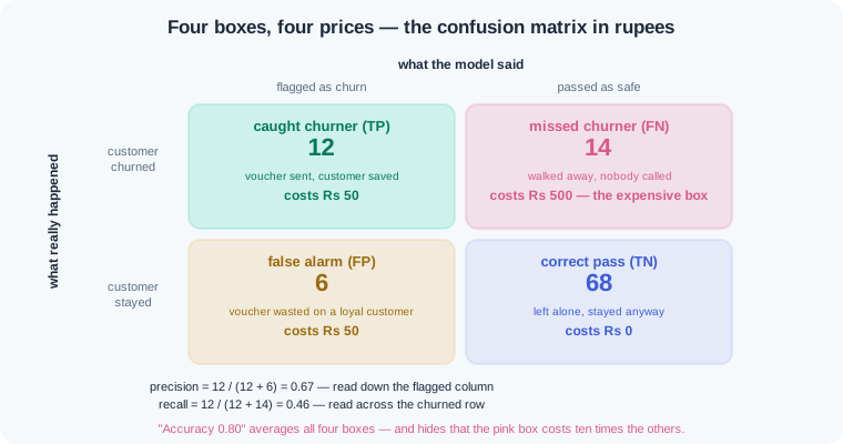
Two honest scores come straight from the boxes. Precision — of everything the model flagged, the share that was truly positive. Recall — of everything truly positive, the share the model caught. They pull against each other like two ends of a rope, and the decision threshold from 1.3 is that rope. Lower the gate and recall rises while precision falls; raise the gate and they trade places.
Which end of the rope should win depends on which mistake hurts more. Fraud and medical screening fear the miss, so recall leads: a missed fraud costs lakhs, a missed illness costs far more. A spam filter fears the false alarm, so precision leads: one real client email buried in spam can cost a deal. There is no best metric in general. There is only the best metric for this problem's costs.
F1 — the harmonic mean of precision and recall, a single number that drops sharply when the two drift apart. Managers like it because it fits in one cell of a slide. Trust it when both mistakes cost about the same, and doubt it when they do not. An F1 of 0.55 can hide a recall of 0.31 or a precision of 0.31, which are very different disasters. When costs differ, sweep the threshold and show the pairs.
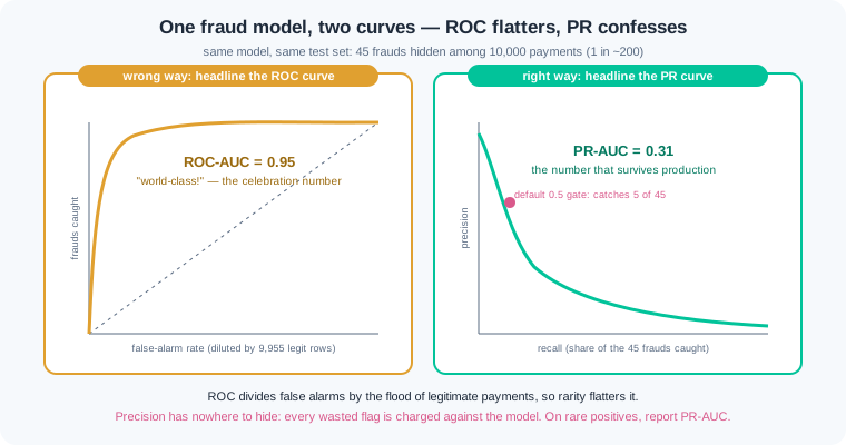
A threshold sweep tries many gates and records precision and recall at each one. Plotted together, the pairs form the precision-recall curve — the model's full menu of trade-offs. Two famous single numbers score ranking quality across all gates at once. ROC-AUC measures how often the model ranks a random positive above a random negative. PR-AUC — the area under the precision-recall curve, the version that stays honest when positives are rare.
Here is the contrast that catches freshers. The wrong way: report "ROC-AUC 0.95" on a one-in-200 fraud table and call the model brilliant. ROC's false-alarm axis divides by the flood of legitimate rows, so even thousands of false alarms barely dent it. The right way: print PR-AUC beside it and show the sweep — the same model scores 0.31 and catches 5 frauds out of 45 at the default gate. One model, two stories; one flatters, one tells the truth.
Regression needs its own rulers. MAE is the average size of a miss in real units, minutes or rupees, every row counted equally. RMSE squares each miss before averaging, so one giant error can dominate the whole score. Read them together: when RMSE towers over MAE, an outlier is hiding in your errors, and your next move is to go look at that row. R² from 1.3 keeps its meaning — the share of the swing explained — and inherits the same outlier warning.
A probability also makes a quiet promise: calibration — when the model says 0.8, close to 80 percent of such cases should truly be positive. A model can rank customers well and still break that promise, like a weather app whose "80 percent rain" days stay dry. Rupee decisions multiply probabilities by money, so test the promise before you spend on it: bucket the predictions and compare each bucket's claim with what happened.
Choose the metric with the business, in rupees, before any modelling. A cost matrix prices each box of the confusion matrix, and the best threshold is whichever gate is cheapest — the sum you started in 1.3. Then report honestly, three things every time: the do-nothing baseline, the chosen metric at the chosen gate, and the uncertainty — how far the number moves across seeds or splits. A score reported without a baseline is a claim, not evidence.
Work inside ai-lab; everything runs on the scikit-learn you installed in 1.2. We stay in the seeded churn world from 1.3 — same customers, same model — and finally give its numbers the reading they deserve.
The scorecard behind 0.80. Rebuild the churn pipeline, then ask for the four boxes instead of one score:
import numpy as np
import pandas as pd
from sklearn.linear_model import LogisticRegression
from sklearn.model_selection import train_test_split
from sklearn.pipeline import make_pipeline
from sklearn.preprocessing import StandardScaler
from sklearn.metrics import confusion_matrix, classification_report

rng = np.random.default_rng(42)
n = 400
customers = pd.DataFrame({
    "orders_last_90d": rng.poisson(6, size=n),
    "days_since_last_order": rng.integers(1, 120, size=n),
    "avg_order_value": rng.integers(120, 900, size=n),
})
risk = (-3.0 + 0.07 * customers["days_since_last_order"]
        - 0.5 * customers["orders_last_90d"])
customers["churned"] = (rng.random(n) < 1 / (1 + np.exp(-risk))).astype(int)

feats = ["orders_last_90d", "days_since_last_order", "avg_order_value"]
Xc_train, Xc_test, yc_train, yc_test = train_test_split(
    customers[feats], customers["churned"],
    test_size=0.25, random_state=42, stratify=customers["churned"])

churn_model = make_pipeline(StandardScaler(), LogisticRegression())
churn_model.fit(Xc_train, yc_train)
pred = churn_model.predict(Xc_test)

print(confusion_matrix(yc_test, pred))
print(classification_report(yc_test, pred, target_names=["stayed", "churned"]))
[[68  6]
 [14 12]]
              precision    recall  f1-score   support

      stayed       0.83      0.92      0.87        74
     churned       0.67      0.46      0.55        26

    accuracy                           0.80       100
   macro avg       0.75      0.69      0.71       100
weighted avg       0.79      0.80      0.79       100
Read the matrix cell by cell, in business words. Top-left 68: correct passes — customers the model left alone who did stay. Top-right 6: false alarms — vouchers about to be wasted on loyal customers. Bottom-left 14: missed churners — the expensive box, customers walking away unflagged. Bottom-right 12: caught churners — the model's actual wins. Now the report: the churned row says precision 0.67 (of 18 flags, 12 were right — 12 ÷ 18) and recall 0.46 (of 26 real churners, it caught 12 — 12 ÷ 26). support is the row count per class: 74 versus 26, the imbalance itself. The 0.80 accuracy you met in 1.3 was the average of one strong story (stayed, recall 0.92) and one weak one (churned, recall 0.46) — and the weak one is the class the business cares about.
The gate as a dial, now with F1. Sweep the threshold and watch the rope pull:
from sklearn.metrics import precision_score, recall_score, f1_score

probs = churn_model.predict_proba(Xc_test)[:, 1]
print(f"{'cutoff':>6s} {'flagged':>8s} {'precision':>10s} {'recall':>7s} {'F1':>6s}")
for cut in [0.3, 0.5, 0.7]:
    p = (probs >= cut).astype(int)
    print(f"{cut:6.1f} {p.sum():8d} {precision_score(yc_test, p):10.2f}"
          f" {recall_score(yc_test, p):7.2f} {f1_score(yc_test, p):6.2f}")
Output, three rows: 0.3 33 0.52 0.65 0.58, then 0.5 18 0.67 0.46 0.55, then 0.7 10 0.80 0.31 0.44. The probabilities never changed — only the gate moved, and precision and recall traded places exactly as the rope predicts. Notice F1 crowns 0.3 as the "best" gate (0.58). But F1 assumed both mistakes cost the same, and nobody asked the retention team. Hold that thought for the last block, where rupees will pick the gate instead.
ROC versus PR on rare fraud — the flattery gap, measured. A bigger, nastier world: 40,000 UPI-style payments, about one fraud in 200:
from sklearn.metrics import roc_auc_score, average_precision_score

rng = np.random.default_rng(7)
n = 40000
fraud = (rng.random(n) < 0.005).astype(int)          # ~1 in 200
payments = pd.DataFrame({
    "amount": np.where(fraud == 1,
                       rng.integers(4000, 20000, size=n),
                       rng.integers(50, 15000, size=n)),
    "new_device": np.where(fraud == 1, rng.random(n) < 0.70,
                           rng.random(n) < 0.08).astype(int),
    "night_txn": np.where(fraud == 1, rng.random(n) < 0.60,
                          rng.random(n) < 0.15).astype(int),
    "fraud": fraud,
})

ffeats = ["amount", "new_device", "night_txn"]
Xf_train, Xf_test, yf_train, yf_test = train_test_split(
    payments[ffeats], payments["fraud"],
    test_size=0.25, random_state=42, stratify=payments["fraud"])

fraud_model = make_pipeline(StandardScaler(), LogisticRegression())
fraud_model.fit(Xf_train, yf_train)
fprobs = fraud_model.predict_proba(Xf_test)[:, 1]

print("ROC-AUC:", round(roc_auc_score(yf_test, fprobs), 2))
print("PR-AUC :", round(average_precision_score(yf_test, fprobs), 2))
for cut in [0.1, 0.3, 0.5]:
    p = (fprobs >= cut).astype(int)
    caught = ((p == 1) & (yf_test == 1)).sum()
    print(f"cutoff {cut:.1f}  flagged {p.sum():4d}"
          f"  caught {caught:2d} of {yf_test.sum()}")
Output: ROC-AUC: 0.95, then PR-AUC : 0.31, then the sweep — cutoff 0.1 flagged 52 caught 16 of 45, cutoff 0.3 flagged 13 caught 7 of 45, cutoff 0.5 flagged 5 caught 5 of 45. Sit with that gap. The ROC number says world-class; the PR number says weak; the sweep says the default gate catches 5 frauds out of 45 while 9,955 legitimate rows pad the ROC score's false-alarm axis. On rare positives, PR-AUC is the honest headline, and average_precision_score is how sklearn spells it. This exact gap, celebrated in a real review meeting, is WR-067.
MAE versus RMSE — one festival day changes everything. Back to Karan's Guwahati delivery line from 1.3, plus one bad day:
from sklearn.linear_model import LinearRegression
from sklearn.metrics import (mean_absolute_error,
                             root_mean_squared_error, r2_score)

rng = np.random.default_rng(7)
n = 400
deliveries = pd.DataFrame({
    "distance_km": rng.uniform(1, 12, n).round(1),
    "items": rng.integers(1, 15, n),
    "order_value": rng.integers(100, 900, n),
})
deliveries["minutes"] = (14 + 2.0 * deliveries["distance_km"]
                         + 0.9 * deliveries["items"]
                         + 0.02 * deliveries["order_value"]
                         + rng.normal(0, 3, n)).round(1)

features = ["distance_km", "items", "order_value"]
X_train, X_test, y_train, y_test = train_test_split(
    deliveries[features], deliveries["minutes"],
    test_size=0.25, random_state=42)

lin = LinearRegression().fit(X_train, y_train)
pred = lin.predict(X_test)
print("normal week    MAE:", round(mean_absolute_error(y_test, pred), 1),
      " RMSE:", round(root_mean_squared_error(y_test, pred), 1),
      " R2:", round(r2_score(y_test, pred), 2))

y_festival = y_test.copy()
y_festival.iloc[0] = 180.0        # one Durga Puja traffic jam
print("festival week  MAE:", round(mean_absolute_error(y_festival, pred), 1),
      " RMSE:", round(root_mean_squared_error(y_festival, pred), 1),
      " R2:", round(r2_score(y_festival, pred), 2))
print((y_festival - pred).round(1).abs().sort_values(ascending=False).head(3))
Output: normal week MAE: 2.3 RMSE: 3.0 R2: 0.9, then festival week MAE: 3.8 RMSE: 14.5 R2: 0.21, then the three largest misses — 142.3, 7.6, 7.5. One row out of 100 moved RMSE from 3.0 to 14.5 and crushed R² from 0.9 to 0.21, while MAE barely stirred. Neither metric is lying: MAE says a typical delivery is still fine, RMSE screams that one delivery was a disaster. The gap between them is the signal — when RMSE towers over MAE, print the sorted residuals and go find the row before you touch the model. A team that skipped that step is WR-068.
Rupees pick the gate. The cost matrix from 1.3's retention world — voucher ₹50 per flag, missed churner ₹500 — applied to the whole sweep:
print(f"{'cutoff':>6s} {'flagged':>8s} {'missed':>7s} {'cost':>8s}")
best = None
for cut in [0.05, 0.1, 0.3, 0.5, 0.7, 0.9]:
    p = (probs >= cut).astype(int)
    tn, fp, fn, tp = confusion_matrix(yc_test, p).ravel()
    cost = 50 * (tp + fp) + 500 * fn        # vouchers sent + churners lost
    best = (cut, cost) if best is None or cost < best[1] else best
    print(f"{cut:6.2f} {tp + fp:8d} {fn:7d} {cost:8,d}")
print("cheapest gate:", best[0], "at Rs", format(best[1], ","))
Output, one row per gate: 0.05 64 0 3,200, 0.10 55 2 3,750, 0.30 33 9 6,150, 0.50 18 14 7,900, 0.70 10 18 9,500, 0.90 3 23 11,650, then cheapest gate: 0.05 at Rs 3,200. This is exercise 1.3-3's answer wearing its proper clothes: each confusion-matrix box got a price, and the sweep became a bill. F1 voted for 0.3; the rupees vote for 0.05, at less than half the cost of the 0.5 default. When metric and money disagree, money was the metric all along — F1 was a stand-in nobody priced. Agreeing on this table with the business before modelling is the whole lesson of WR-069.
Work inside ai-lab. Every world is seeded, so where a check states a number, your number must match it exactly.
Read the scorecard, cell by cell. Create churn_scorecard.py. Rebuild the watch block's churn world and pipeline exactly (seed 42, same draw order, same split). Print the confusion matrix and the classification report at the default gate. Then compute precision, recall and F1 for the churned class by hand — plain arithmetic on the four matrix cells, no sklearn metric calls — and print your hand values beside the report's values. Finish with four comment lines, one per cell, each naming the business meaning and the count (caught churner, false alarm, missed churner, correct pass). Check: the matrix prints [[68 6],[14 12]]; your hand-computed values print 0.67 (12 of 18 flags), 0.46 (12 of 26 churners) and 0.55, matching the report to two decimals; the four comment lines carry the counts 12, 6, 14 and 68 against the correct business names.
The metric memo. Three teams ask you to pick their evaluation metric. Write metric_memo.md with one short section per team. (a) UPI fraud screening: one fraud in 200 payments, a missed fraud costs about ₹15,000, a false alarm costs a 30-second manual review. (b) A spam filter for a sales inbox: one real client mail lost to the spam folder can cost a deal worth lakhs. (c) NBFC loan approval: approving a future defaulter loses about ₹40,000; wrongly rejecting a good customer loses about ₹4,000 of margin. For each team: name the headline metric, say which direction you would push the threshold from 0.5 and why, and defend the choice in at most three sentences a non-technical head can follow. The word "accuracy" may appear only inside a sentence explaining why it is not the headline. Check: section (a) leads with recall or PR-AUC and pushes the gate down; section (b) leads with precision and pushes the gate up; section (c) prices both mistakes, notes the 10-to-1 cost ratio, and argues for a low gate on expected rupee cost; no section uses accuracy as its headline metric.
The flattery gap, staged by you. Create flattery_gap.py. Rebuild the watch block's payment world exactly (seed 7, n=40000, draws in the same order) and refit the fraud pipeline. Print: ROC-AUC and PR-AUC; the sweep at cutoffs 0.1, 0.3 and 0.5 with flagged and caught counts; the catch count of a top-200 review queue (sort all test rows by predicted probability, take the 200 highest, count true frauds); and the accuracy of a do-nothing rule that predicts "not fraud" for every row, rounded to three decimals. Close with a two-line verdict naming the number you would put in a leadership email and the number you would refuse to headline. Check: ROC-AUC prints 0.95 and PR-AUC prints 0.31; the 0.5 gate catches 5 of 45 test frauds; the top-200 queue catches 29 of 45; the do-nothing accuracy prints 0.996; the verdict headlines PR-AUC (with the sweep) and refuses ROC-AUC and accuracy.
Find the lie. Four results land in your inbox before a Monday review; each hides one trap from this module. (A) "Churn model v2 hits 96.1 percent accuracy" — the attached test set has 960 stayed and 40 churned. (B) "Fraud v3 scores ROC-AUC 0.97, ready to ship" — fraud rate one in 250, no other number given. (C) "Delivery model healthy: average miss is only 3.8 minutes" — the attached errors file contains one 142-minute miss. (D) "New loan model reaches 100 percent accuracy" — a footnote admits it was scored on the rows it trained on. Write lie_detector.md: for each result, one sentence naming the trap, one sentence naming the single artefact you would demand, and one sentence stating the honest fix. Then prove trap A in lie_check.py: with np.random.default_rng(5), build 1,000 labels where churn probability is 0.04, and print the accuracy of always predicting "stayed", rounded to two decimals. Check: the four traps map to accuracy-on-imbalance, ROC-on-rare-positives, an outlier hidden by quoting MAE alone, and train-set evaluation; the four demanded artefacts are a confusion matrix, PR-AUC with a threshold sweep, RMSE beside MAE with the sorted residuals, and a score on an untouched test set; lie_check.py prints a value of 0.95 or higher without any model at all.
Three evaluation failures cover most of what this lesson meets in production. Each has a War Room entry with the full diagnosis path:
- WR-067 — the AUC that flattered. A fraud model wore a 0.95 ROC-AUC on one-in-200 data while catching almost nothing at any usable gate; PR-AUC and a threshold sweep exposed the gap before the celebration became a launch.
- WR-068 — the RMSE ambush. One festival-day outlier sent RMSE from 3 to 14 and a team spent a sprint "fixing" a model that was never broken; MAE beside RMSE plus one sorted residual table found the single guilty row.
- WR-069 — the metric nobody agreed on. Data science maximised F1 while operations was judged on wasted vouchers, so a "great" model was hated on the floor; the fix was a rupee cost matrix agreed with stakeholders before modelling, not after.
Accuracy is one number, and on imbalanced data it flatters models that do almost nothing. The confusion matrix shows the four outcomes by name, and precision and recall score the two mistakes that matter. The decision threshold trades those two against each other, so sweep it and price every gate in rupees before choosing. On rare positives report PR-AUC, because ROC-AUC can stay high while the model misses nearly everything. For number predictions read MAE and RMSE together to catch hiding outliers, and always report the baseline and the uncertainty beside your headline metric.
- UPI fraud engines at Indian payment companies are judged on PR curves and review-queue catch rates, never on accuracy — at one fraud in hundreds of payments, accuracy praises doing nothing.
- Health screening camps, like diabetic retinopathy drives, set thresholds recall-first: a false alarm costs one extra check-up, a miss costs a patient — the exact tug-of-war from this module.
- Quick-commerce logistics teams track MAE and worst-day residuals on delivery-time models, because festival spikes taught them that a single RMSE headline misleads twice a year.
Answer these before opening the gate assessment. Each question names its type.
type=output-prediction— A churn test set has 26 churners among 100 rows. At the current gate the model flags 20 customers, of whom 13 are real churners. Predict the four confusion-matrix cells and the precision and recall the report will print for the churned class.type=interpretation— A fraud model prints ROC-AUC 0.95 and PR-AUC 0.31 on a one-in-200 table. Explain what each number measures, why they disagree so sharply here, and which one you would put in the headline of your report.type=debug— After a festival week, a delivery model's RMSE jumps from 3.0 to 14.5 while MAE only moves from 2.3 to 3.8, and a teammate declares the model broken everywhere. Name the likelier cause, the one table you would print to confirm it, and what you would report instead.type=scenario-judgement— Your team tuned the churn threshold to maximise F1, but the retention head is judged on wasted vouchers and calls the model unusable. Judge whose metric should win, and describe the one meeting and one artefact that would have prevented the fight.type=trade-off— Compare reporting a single summary number (F1 or ROC-AUC) against reporting a full threshold sweep with a rupee cost column. Give one concrete advantage and one concrete cost of each, and name the audience for which each is the right choice.
Explain to a friend who runs a kirana shop why a watchman who was "right 99 percent of the time" might still be a useless watchman, and what four counts you would ask for instead of that one number. Use at most 4 sentences and no word fancier than "count". If your friend can say which mistake — a false alarm or a missed thief — hurts their shop more, you own this module.