CV, tuning, model selection
Friday review at a Kanpur NBFC. Anjali brings one slide: her boosted loan model wins, 0.86 against 0.83. Her lead reruns the notebook with a different split seed, and the winner flips. Same data, same two models — now the plain model leads. Which slide is true? Neither, says the lead. One split is one exam, and exams carry luck. By the next review, Anjali averages five exams, tunes with a budget, and keeps one sealed paper for the end.
- "Which number goes on the slide?" is a daily question in every ML team, and this module gives you the professional answer: mean ± std across folds, plus one sealed test score.
- "Your CV said 0.86 and production says 0.71 — what happened?" is a standard interview probe at Indian fintechs, and the validation-set trap in this lesson is the full story behind it.
- Every later phase reuses today's ritual: deep-learning runs, RAG evaluations and A/B decisions all pick winners by averaged scores and a final set touched once.
Module 1.7 taught you to keep the test set honest. This module asks a harder question: how much can one split be trusted at all? Below, the sealed Pipeline from 1.6 meets five different random splits and scores 0.80, 0.86, 0.83, 0.81 and 0.81. Nothing about the model changed — only the shuffle did. A single split is one exam, and exams carry luck.
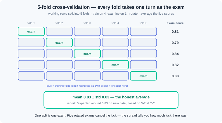
Cross-validation — splitting the training data into k folds and letting each fold take one turn as the exam. The model trains k times, each time on the other folds, and the k scores are averaged. The average cancels split luck, and the spread shows how much luck there was. Use k=5 as the default, and move to k=10 when rows are scarce and you can pay double the fits. For classification, scikit-learn stratifies the folds by default, so 1.7's class-balance rule holds inside every fold.
Two kinds of numbers live inside every model, and interviews check that you can separate them. Parameters are the values fit learns from data — the weights in a logistic model, the split points in a tree. A hyperparameter — a knob you set before training, like C, max_depth or learning_rate. No fit call can learn a hyperparameter; something outside the training loop must choose it. That chooser is a search, and the search needs honest scores.
GridSearchCV — the scikit-learn tool that tries every combination in a parameter grid and cross-validates each one. It is thorough and it is costly: combinations multiply, and each one costs k fits. RandomizedSearchCV — the budgeted cousin that samples a fixed number of combinations from the same space. On big spaces, random sampling usually finds a near-best setting in a fraction of the fits, because only a few knobs matter on most tables. Grid suits small, cheap spaces; random suits everything larger.
Now the trap this module exists to name. Tune forty times against one validation split and the split stops being an exam — you have memorised its questions. The score climbs while the model does not improve, which is overfitting the validation set itself. The cure is a final test set that you touch exactly once, after all tuning ends. For interviews, name the stronger version too: nested cross-validation — an outer CV loop that scores the entire tuning ritual, folds within folds.
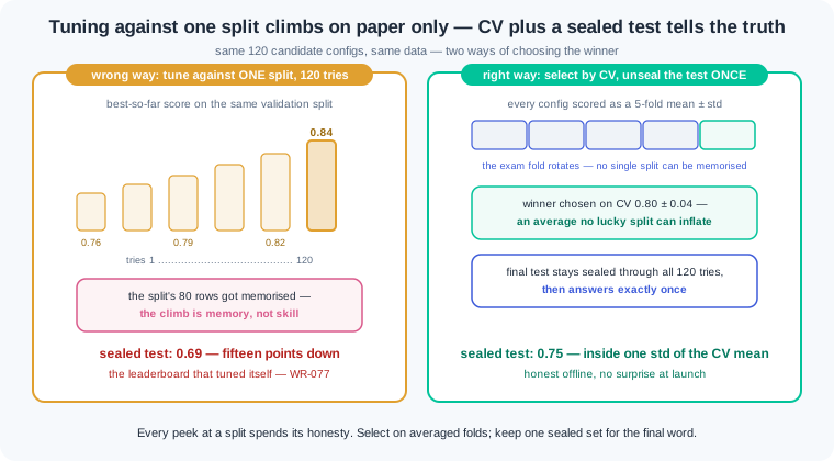
The wrong way and the right way sit side by side in that picture. Wrong: keep tuning against the same split until the number looks good, then report that number. Right: select with cross-validation, and spend the sealed test once for the final line of the report. Every extra peek at the test set quietly turns it into another validation split.
Tuning must include the preprocessing, and 1.6's Pipeline makes that possible. Pass the whole Pipeline to the search, and every fold fits its own scaler and encoder on that fold's training rows only. Scale before the search instead, and every fold has already seen its exam rows — 1.7's preprocessing leak, reborn inside tuning. The search can even tune preparation choices, like which scaler to use, beside model knobs. One object, one honest search.
Selection at the end is a table, not a feeling. List each candidate's CV mean and std, then apply the working rule: among models within one std of the best, pick the simplest. Simple models are cheaper to serve, easier to defend in review, and harder to break. Then write the line the industry expects: expected around 0.83 on new data, based on 5-fold CV. The final test score, touched once, sits beside it as proof.
Work inside ai-lab. The churn world stays in Ludhiana: same seeded table as 1.6, same sealed Pipeline — wrapped in a builder function so every experiment gets a fresh, unfitted copy.
Split luck, measured. Rebuild the world, then give the identical pipeline five different random splits:
import numpy as np
import pandas as pd
from sklearn.linear_model import LogisticRegression
from sklearn.model_selection import train_test_split
from sklearn.pipeline import Pipeline
from sklearn.preprocessing import (StandardScaler, MinMaxScaler,
                                   FunctionTransformer, OneHotEncoder)
from sklearn.compose import ColumnTransformer

rng = np.random.default_rng(42)
n = 500
snapshot = pd.Timestamp("2026-06-30")
customers = pd.DataFrame({
    "city": rng.choice(["Ludhiana", "Jalandhar", "Amritsar",
                        "Patiala", "Bathinda"], size=n),
    "monthly_income": rng.integers(18000, 120000, size=n),
    "orders_last_90d": rng.poisson(6, size=n),
    "avg_order_value": rng.integers(120, 900, size=n),
})
customers["last_order_date"] = snapshot - pd.to_timedelta(
    rng.integers(1, 120, size=n), unit="D")
spend_share = (customers["avg_order_value"]
               * customers["orders_last_90d"] / 3) / customers["monthly_income"]
days_since = (snapshot - customers["last_order_date"]).dt.days
salary_week = (customers["last_order_date"].dt.day <= 7).astype(int)
risk = (-3.0 + 0.05 * days_since - 25 * spend_share
        - 1.3 * salary_week - 0.15 * customers["orders_last_90d"])
customers["churned"] = (rng.random(n) < 1 / (1 + np.exp(-risk))).astype(int)

raw_feats = ["monthly_income", "orders_last_90d", "avg_order_value"]

def add_features(df):
    out = df.copy()
    out["days_since_last_order"] = (snapshot - out["last_order_date"]).dt.days
    out["spend_share"] = (out["avg_order_value"]
                          * out["orders_last_90d"] / 3) / out["monthly_income"]
    out["salary_week_order"] = (out["last_order_date"].dt.day <= 7).astype(int)
    return out

eng_feats = raw_feats + ["days_since_last_order",
                         "spend_share", "salary_week_order"]

def make_churn_pipe():
    return Pipeline([
        ("features", FunctionTransformer(add_features)),
        ("prep", ColumnTransformer([
            ("city", OneHotEncoder(handle_unknown="ignore"), ["city"]),
            ("num", StandardScaler(), eng_feats),
        ])),
        ("model", LogisticRegression(max_iter=1000)),
    ])

X = customers.drop(columns="churned")
y = customers["churned"]

scores = []
for seed in range(5):
    X_tr, X_te, y_tr, y_te = train_test_split(
        X, y, test_size=0.25, random_state=seed, stratify=y)
    pipe = make_churn_pipe()
    pipe.fit(X_tr, y_tr)
    scores.append(pipe.score(X_te, y_te))
    print(f"split seed {seed}   accuracy: {scores[-1]:.2f}")
print(f"spread: {min(scores):.2f} to {max(scores):.2f}")
split seed 0   accuracy: 0.80
split seed 1   accuracy: 0.86
split seed 2   accuracy: 0.83
split seed 3   accuracy: 0.81
split seed 4   accuracy: 0.81
spread: 0.80 to 0.86
Six accuracy points of spread, and the model never changed — only the shuffle did. This is 1.4's "which model wins" question with the rug pulled away: on seed 1 you would brag about 0.86, on seed 0 you would apologise for 0.80, and both claims describe the same pipeline. Any comparison built on one split is a comparison of luck. This is the failure WR-076 documents from production.
The honest average. Seal a final test set FIRST — it stays untouched until the last fence — then let cross_val_score average five exams on the working rows:
from sklearn.model_selection import cross_val_score

X_work, X_final, y_work, y_final = train_test_split(
    X, y, test_size=0.2, random_state=42, stratify=y)

cv_scores = cross_val_score(make_churn_pipe(), X_work, y_work, cv=5)
print("fold scores:", np.round(cv_scores, 2))
print(f"mean: {cv_scores.mean():.2f}   std: {cv_scores.std():.2f}")
print(f"report: expected around {cv_scores.mean():.2f} on new data, "
      f"based on 5-fold CV (+/- {cv_scores.std():.2f})")
Output: fold scores: [0.81 0.79 0.84 0.82 0.88], then mean: 0.83 std: 0.03, then the report line — expected around 0.83 on new data, based on 5-fold CV (+/- 0.03). Read the parts. Each fold score is one exam where 80 percent of the working rows trained and 20 percent examined; because y is binary, cv=5 quietly used stratified folds, keeping 1.7's class-balance rule. The mean is the number you report, and the std says one split can wander a few points — exactly the wobble the first fence measured. Note what the pipeline bought us: every fold fitted its own scaler and encoder on that fold's training rows, so no preprocessing leak crossed a fold boundary.
One search over the whole Pipeline. GridSearchCV addresses any step with double underscores — model__C reaches the model's knob, prep__num swaps the numeric scaler — so preparation and model are tuned together, inside the folds:
from sklearn.model_selection import GridSearchCV

grid = GridSearchCV(make_churn_pipe(), param_grid={
    "prep__num": [StandardScaler(), MinMaxScaler()],
    "model__C": [0.01, 0.1, 1, 10],
}, cv=5)
grid.fit(X_work, y_work)

print("combinations tried:", len(grid.cv_results_["params"]))
print("total fits:", len(grid.cv_results_["params"]) * grid.n_splits_)
print("best params:", grid.best_params_)
i = grid.best_index_
print(f"best CV score: {grid.best_score_:.2f} "
      f"(+/- {grid.cv_results_['std_test_score'][i]:.2f})")
Output: combinations tried: 8, total fits: 40, best params: {'model__C': 1, 'prep__num': StandardScaler()}, best CV score: 0.83 (+/- 0.03). The arithmetic first: 2 scalers × 4 C values is 8 combinations, and each pays 5 cross-validation fits, so 40 fits total — always run this multiplication before pressing enter (WR-078 is what happens when nobody does). The verdict: defaults were already fine here, C=1 with StandardScaler, and the search proved it for the price of 40 fits. A search that confirms the default is not a failure; it is evidence you could not have claimed before.
When random beats grid. Swap in 1.4's boosted model, whose knobs multiply faster. The full grid costs 240 fits; RandomizedSearchCV samples twelve combinations from the same space for 60:
from sklearn.ensemble import HistGradientBoostingClassifier
from sklearn.model_selection import RandomizedSearchCV

hgb_pipe = Pipeline([
    ("features", FunctionTransformer(add_features)),
    ("prep", ColumnTransformer([
        ("city", OneHotEncoder(handle_unknown="ignore"), ["city"]),
        ("num", "passthrough", eng_feats),
    ])),
    ("model", HistGradientBoostingClassifier(random_state=42)),
])
space = {
    "model__learning_rate": [0.03, 0.06, 0.1, 0.2],
    "model__max_depth": [2, 3, 4, None],
    "model__min_samples_leaf": [10, 20, 40],
}

big_grid = GridSearchCV(hgb_pipe, space, cv=5)
big_grid.fit(X_work, y_work)
print(f"grid   : {len(big_grid.cv_results_['params']) * 5} fits"
      f"   best CV: {big_grid.best_score_:.2f}")

rand = RandomizedSearchCV(hgb_pipe, space, n_iter=12, cv=5, random_state=42)
rand.fit(X_work, y_work)
print(f"random : {len(rand.cv_results_['params']) * 5} fits"
      f"   best CV: {rand.best_score_:.2f}")
print("random best params:", rand.best_params_)
Output: grid : 240 fits best CV: 0.82, then random : 60 fits best CV: 0.82, then random best params: {'model__min_samples_leaf': 40, 'model__max_depth': 2, 'model__learning_rate': 0.1}. Same best score, one quarter of the compute — the space is 4 × 4 × 3 = 48 combinations, and twelve random samples were enough to land within rounding of the exhaustive answer. Notice the boosted pipeline's prep keeps the numerics as "passthrough": trees split on thresholds, so scaling buys them nothing. On an ordinary laptop, this fence is the difference between minutes and an afternoon; at WR-078's six-knob scale, between an afternoon and a week.
The final honest report. Compare the two searches on CV terms, pick like a professional, and only then unseal the final test — once:
li, bi = grid.best_index_, big_grid.best_index_
print(f"logistic pipeline  CV: {grid.best_score_:.2f} "
      f"+/- {grid.cv_results_['std_test_score'][li]:.2f}")
print(f"boosted  pipeline  CV: {big_grid.best_score_:.2f} "
      f"+/- {big_grid.cv_results_['std_test_score'][bi]:.2f}")

final_model = grid.best_estimator_          # simplest within one std
print(f"final test (touched once): {final_model.score(X_final, y_final):.2f}")
Output: logistic pipeline CV: 0.83 +/- 0.03, boosted pipeline CV: 0.82 +/- 0.04, final test (touched once): 0.81. The boosted model sits within one std of the logistic one, so the one-std rule says: take the simpler machine. grid.best_estimator_ is that pipeline already refitted on all working rows — GridSearchCV refits the winner automatically. The sealed test answers 0.81, two points under the CV mean and inside its std, which is what honesty looks like: no collapse, no miracle. Anjali's slide now reads "expected around 0.83 on new data, based on 5-fold CV; sealed test agreed at 0.81" — and that sentence survives any reviewer, any reseed, and any interview.
Work inside ai-lab. Every world is seeded: where a check states a number, your number must match it exactly.
The tuning tournament, on loans. Anjali's NBFC world, three model families, one honest table. In tuning_tournament.py, with np.random.default_rng(21) and n=900, build a loan table with columns drawn in this exact order: city chosen from Kanpur, Agra, Jhansi, Prayagraj; monthly_income integers 25,000–150,000; emi integers 2,000–40,000; months_on_book integers 3–48; bounced_payments Poisson(mean 1.0). Then defaulted = 1 with probability sigmoid(-4.8 + 9*(emi/monthly_income) + 15*(bounced_payments/months_on_book)), drawn with one rng.random(900) call. Seal a final test set immediately: test_size 0.2, random_state=42, stratified — it is touched exactly once, at the end. Write one pipeline builder make_pipe(model): a FunctionTransformer adding emi_ratio (emi over income) and bounce_rate (bounces over months), a ColumnTransformer sending city to OneHotEncoder(handle_unknown="ignore") and the six numerics to StandardScaler, then the model. Run three searches with cv=5 on the working rows: (a) GridSearchCV on logistic — model__C in [0.01, 0.1, 1, 10] × model__class_weight in [None, "balanced"]; (b) GridSearchCV on RandomForestClassifier(n_estimators=200, random_state=42) — model__max_depth in [3, 6, None] × model__min_samples_leaf in [2, 10, 30]; (c) RandomizedSearchCV on HistGradientBoostingClassifier(random_state=42) — model__learning_rate in [0.05, 0.1, 0.2], model__max_depth in [2, 3, None], model__min_samples_leaf in [10, 20, 40], n_iter=10, random_state=42. Print one honest table — family, best CV mean, std, fits — then name every family within one std of the best, pick the simplest of them, and score the sealed test once with that search's best_estimator_. Close with the report sentence in the lesson's language. Check: the default rate prints 0.31; the table reads logistic 0.85 ± 0.02 with 40 fits, forest 0.84 ± 0.03 with 45 fits, boosted 0.83 ± 0.01 with 50 fits — 135 fits in total; logistic and forest are within one std of the best, so the pick is logistic (C=10, class_weight None); the sealed test prints 0.84, inside one std of the CV mean; your report sentence says expected around 0.85 on new data, based on 5-fold CV.
Tune against one split, then apologise. Reproduce the validation-set trap, measure the damage, then repair it with CV. In val_overfit.py, with np.random.default_rng(11) and n=400, draw in this exact order: monthly_income integers 20,000–120,000; emi integers 2,000–35,000; bounced_payments Poisson(mean 0.8); then a 400 × 12 block of rng.normal(0, 1) noise stored as columns noise0…noise11. Then defaulted = 1 with probability sigmoid(-3.6 + 8*(emi/monthly_income) + 0.8*bounced_payments), one rng.random(400) call. Split twice with seed 42, stratified: first seal a final test set (test_size 0.2), then cut the rest into train and ONE validation split (test_size 0.25). Build 120 candidate configs: for trial in 0–119, seed np.random.default_rng(trial), keep each of the 15 columns with probability 0.5 (force column 0 if none survive), and draw C from [0.01, 0.1, 1.0, 10.0, 100.0]. Round one — the wrong way: fit make_pipeline(StandardScaler(), LogisticRegression(max_iter=1000, C=C)) on the train rows for every config, score on the single validation split, keep the best val score, then unseal the final test for its winner. Round two — the honest way: score every config with cross_val_score(cv=5) on train+validation combined, pick the best mean, refit, and score the sealed test with it. Print both rounds side by side and finish with three sentences: why round one's winner fell hardest, what its noise-column count tells you, and which single habit prevents the fall. Check: the default rate prints 0.42 and the row counts print 240 train, 80 validation, 80 final test; round one's winner (trial 75, 6 features of which 4 are noise, C=10.0) prints best val 0.84 and final test 0.69 — a fifteen-point apology; round two's winner (trial 26, C=10.0) prints CV 0.80 ± 0.04 and final test 0.75 — the CV estimate misses by five points and stays within about one std, while the one-split estimate missed by fifteen; your sentences say the one-split winner memorised the 80 validation rows through lucky noise columns, and the habit is selecting on averaged folds, never on one split you have peeked at 120 times.
The k drill, and the folds that lose their churners. In k_drill.py, with np.random.default_rng(5) and n=400, draw orders_last_90d Poisson(6), then days_since_last_order integers 1–120, then churned = 1 with probability sigmoid(-4.6 + 0.045*days_since_last_order - 0.25*orders_last_90d) — a rare-churn world. Model: make_pipeline(StandardScaler(), LogisticRegression(max_iter=1000, class_weight="balanced")). Part (a): using KFold(n_splits=5) and StratifiedKFold(n_splits=5), print how many churners land in each test fold under each splitter. Part (b): run cross_val_score with scoring="recall" for k = 3, 5 and 10, printing mean, std and the number of fits for each. Part (c): close with a three-line memo — one line choosing k for this table and defending the cost, one line explaining why the k=10 std looks scarier without the model being worse, and one line reporting the k=5 result in the lesson's language. Check: the world holds 39 churners in 400 rows (rate 0.10); plain KFold's folds hold [6, 10, 12, 4, 7] churners while stratified folds hold [7, 8, 8, 8, 8] — one plain fold nearly lost half its positive class; the recall table prints k=3 mean 0.77 std 0.06, k=5 mean 0.76 std 0.16, k=10 mean 0.77 std 0.18; your memo says the mean barely moves with k while smaller test folds make per-fold recall jumpy (four churners per fold at k=10), picks k=5 stratified as the default, and reports expected recall around 0.76, based on 5-fold CV.
Three tuning disasters cover most of what this lesson meets in production. Each has a War Room entry with the full diagnosis path:
- WR-076 — the lucky split. A model was crowned on one 0.86 split, demoed as the winner, and shipped mediocre; five reseeded splits later the "win" was pure shuffle luck, and 5-fold CV before any claim is the fix and the habit.
- WR-077 — the leaderboard that tuned itself. Forty tuning rounds against the same validation set manufactured a 0.92 that was memorisation, not skill; the final test collapsed at launch review, and the cure is selection by CV with a sealed test touched exactly once.
- WR-078 — the grid that never ended. A six-knob full grid launched on a laptop at 6 pm was still at 11 percent the next morning; multiplying the combinations first, sampling with RandomizedSearchCV, searching coarse-to-fine and setting
n_jobs=-1turned days into minutes.
One split is one exam, so its score moves with the shuffle, and cross-validation replaces it with a mean ± std across k folds. Hyperparameters are the knobs you set before training, and GridSearchCV or RandomizedSearchCV chooses them by cross-validated score, with random sampling winning on large spaces. Tuning many rounds against one validation split overfits that split, so the final test set is touched exactly once, after every decision is made. The whole 1.6 Pipeline goes inside the search, so each fold fits its own preprocessing and 1.7's leakage rules keep holding during tuning. Report like a professional: pick the simplest model within one std of the best CV mean, and state that you expect around the CV mean on new data.
- Indian banks and NBFCs re-tune credit scorecards every quarter under audit. The model board reads fold means with spreads, and one sealed sample plays the touched-once test before go-live.
- Kaggle and ML hiring assignments are decided by this module. A public leaderboard is one split, so serious entrants trust their own CV and submit sparingly — the private-leaderboard crash is WR-077 at contest scale.
- GenAI teams tune retrieval settings the same waychunk sizes and thresholds are searched against averaged golden-set folds, and one sealed evaluation set gives the launch number.
Answer these before opening the gate assessment. Each question names its type.
type=output-prediction— AGridSearchCVgets a grid of 4 C values and 2 scalers withcv=5, on 400 working rows. Predict the number of combinations, the total fits, and roughly how many rows each fold's training side holds. Then predict both fit numbers again forcv=10and say what you paid for the extra folds.type=debug— A teammate's search reports best CV 0.97, but the sealed test says 0.62. Their script scales the full table with a fittedStandardScalerbefore the search, and their target encoder was fitted on all rows in week one. Name the two distinct faults, say which one manufactured most of the 0.97, and give the one-object fix that removes both.type=interpretation— A tournament table reads: boosted 0.86 ± 0.05, forest 0.84 ± 0.03, logistic 0.83 ± 0.02. The team wants the boosted model "because it is the biggest number". Read the table back to them with the one-std rule: which families are within one std of the best, what would you pick, and what extra evidence could change your pick?type=scenario-judgement— Demo is Monday. A teammate proposes scoring the sealed test after each of the twelve remaining tuning ideas, "so we always know where we stand". Judge the proposal, name what the test set silently becomes by Friday, and give the version of the plan you would approve.type=trade-off— For a six-knob boosted model on an ordinary laptop, compare a full grid, RandomizedSearchCV with a budget, and a coarse-to-fine sequence of two small searches. Give one concrete strength and one concrete cost of each, and name the fit-count multiplication you would run before choosing.
Explain to a friend who coaches cricket trials why picking a team from one practice match is a gamble: one pitch, one morning, one lucky innings. Cover why five rotated matches with the average score is fairer (cross-validation), why letting a player retake the same trial forty times until he tops it proves memory rather than form (the validation-set trap), and why the selectors keep one final unseen match to confirm the pick (the test touched once). Use at most 4 sentences and no word fancier than "trial match". If your friend can say why the average of five matches beats the best of one, you own this module.