Interpreting models
Monday morning at a Raipur NBFC. Manish's boosted model now scores every loan file, and a rejected shopkeeper is standing at the counter, asking why. The branch head forwards a circular: lenders must give rejected applicants their main reasons, in plain words. Manish opens his notebook and finds an accuracy, a confusion matrix, and no sentence he could print in a letter. The model decides in milliseconds, and nobody in the branch can say what it weighed. By Friday, he must.
- Indian lenders must tell a rejected borrower the main reasons, so a model nobody can explain cannot ship in banking, lending or insurance.
- "Why did your model reject this file?" is a standard fresher interview probe, and importance charts are where most candidates get caught.
- Interpretation is also debugging: split credit, leaks and nonsense features show up in explanations before they show up in production.
A test score says how often the model is right. It never says why, and three audiences need the why. The business will not act on a churn list nobody can defend. You cannot debug a model you cannot read. And a lender must hand a rejected borrower the main reasons, in words the borrower can use.
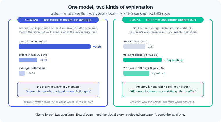
The why comes in two sizes. A global explanation — the story of what drives the model overall, across all customers. A local explanation — the story of why the model gave THIS customer THIS score. A strategy meeting needs the first; a rejection letter needs the second. The same model answers both, with different tools.
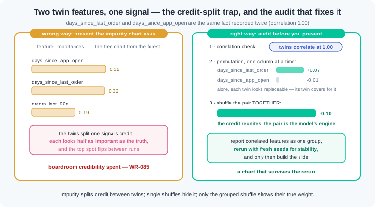
For the global story, 1.4 left you an unpaid debt. The forest's free chart, impurity importance, is measured on training rows and splits credit between correlated features. Our churn table records the same fact twice — days since the last order, and days since the app was opened. Each twin then shows half its true weight, and the top spot flips between reruns. Presenting that chart as-is burned a boardroom in WR-085.
The honest cross-check is permutation importance — shuffle one column on held-out rows and measure how far the score falls. It reads what the model truly depends on, but single-column shuffles have a blind spot: shuffle one twin, and the other covers for it. So the audit has three steps. Check the correlation, shuffle correlated twins together as one group, and rerun with fresh seeds. The group's joint score drop is the signal's true weight.
Global stories also need shape, not only rank. Partial dependence — how the model's average prediction moves as one feature moves, with the others left as they are. scikit-learn sweeps the feature across a grid and averages the model's predictions at each stop. The output reads like a business rule: churn risk sits flat for the first few weeks of silence, then climbs. That shape tells a growth team exactly when the winback message should go out.
For the local story, the industry standard is SHAP — a method that splits one prediction's distance from the average fairly across the features. Start at the average customer, add each feature's push up or down, and you land exactly on this customer's score. A simpler tool gets you far first: swap one of the customer's values to the typical level and watch the prediction move. Both answer the officer's question — what, in this one file, moved the number.
Now the sentence the customer hears. The wrong way is to mail the explainer's raw output: "SHAP value -0.42 on feature emi_ratio" — true, and useless to its reader. The right way is an adverse action sentence — the decision's main reason in plain words, with the customer's own numbers and what would change the outcome. "Your EMIs would take 45% of your monthly income; we approve when this stays under 35%." A letter fails if a non-technical colleague cannot read it aloud and say what the customer should fix.
Three honesty rules guard everything above. Explanations show association, not causation — 1.3's lesson stands: long silence marks churners, but forcing an order will not force loyalty. Explanations of a bad model are confident nonsense, because a chart cannot add skill the test score says is missing. And interpretation never fixes leakage: every tool on this page will crown a leaked column, brilliantly. Check the score and the split discipline before you explain anything.
Work inside ai-lab. This is the seeded churn world from 1.4, with the twin column that staged the importance trap — now we finish that story. Everything runs on scikit-learn; the one optional extra is shap, clearly marked below.
The two importance tables side by side — and the grouped shuffle. Build the world, add the twin, train the forest, then measure importance both ways:
import numpy as np
import pandas as pd
from sklearn.model_selection import train_test_split
from sklearn.ensemble import RandomForestClassifier
from sklearn.inspection import permutation_importance

rng = np.random.default_rng(42)
n = 400
customers = pd.DataFrame({
    "city": rng.choice(["Patna", "Gaya", "Muzaffarpur"], size=n),
    "orders_last_90d": rng.poisson(6, size=n),
    "days_since_last_order": rng.integers(1, 120, size=n),
    "avg_order_value": rng.integers(120, 900, size=n),
})
risk = (-3.0 + 0.07 * customers["days_since_last_order"]
        - 0.5 * customers["orders_last_90d"])
customers["churned"] = (rng.random(n) < 1 / (1 + np.exp(-risk))).astype(int)

feats = ["orders_last_90d", "days_since_last_order", "avg_order_value"]
X_train, X_test, y_train, y_test = train_test_split(
    customers[feats], customers["churned"],
    test_size=0.25, random_state=42, stratify=customers["churned"])

rng2 = np.random.default_rng(0)
X_train = X_train.copy()
X_train["days_since_app_open"] = (
    X_train["days_since_last_order"] + rng2.normal(0, 2, len(X_train))).round(1)
rng3 = np.random.default_rng(1)
X_test = X_test.copy()
X_test["days_since_app_open"] = (
    X_test["days_since_last_order"] + rng3.normal(0, 2, len(X_test))).round(1)

forest = RandomForestClassifier(n_estimators=200, random_state=42)
forest.fit(X_train, y_train)
base_acc = forest.score(X_test, y_test)
print(f"test accuracy: {base_acc:.2f}")

pi = permutation_importance(forest, X_test, y_test,
                            n_repeats=20, random_state=42)
print(f"{'feature':24s} {'impurity':>9s} {'permutation':>12s}")
for name, imp, perm in sorted(
        zip(X_train.columns, forest.feature_importances_, pi.importances_mean),
        key=lambda t: -t[1]):
    print(f"{name:24s} {imp:9.3f} {perm:+12.3f}")

twins = ["days_since_last_order", "days_since_app_open"]
print(f"twin correlation: {X_train[twins].corr().iloc[0, 1]:.2f}")

r = np.random.default_rng(42)
drops = []
for _ in range(20):
    Xs = X_test.copy()
    order = r.permutation(len(Xs))
    for c in twins:
        Xs[c] = Xs[c].to_numpy()[order]
    drops.append(base_acc - forest.score(Xs, y_test))
print(f"shuffle the twin pair together: score drop {np.mean(drops):+.3f}")
Output:
test accuracy: 0.78
feature                   impurity  permutation
days_since_app_open          0.323       -0.014
days_since_last_order        0.320       +0.070
orders_last_90d              0.189       -0.006
avg_order_value              0.168       -0.027
twin correlation: 1.00
shuffle the twin pair together: score drop +0.099
Read the two columns against each other. In 1.4, without the twin, days_since_last_order held 0.555 of impurity credit; here the twins split it 0.323 + 0.320, and the copycat column sits on top. The permutation column then tells a different story — the twin scores a meaningless -0.014, because shuffling it alone lets its partner cover the signal. Neither single number is the truth. The truth is the grouped shuffle at the bottom: kill both twins together and the score drops by 0.099, the pair's real weight. That is the full audit from the figure — correlation printed, singles measured, group shuffled — and it is what WR-085's team wished they had run before the boardroom.
Partial dependence, as a table you can read aloud. How does predicted churn move as silence grows? Sweep one feature, average the predictions:
from sklearn.inspection import partial_dependence

pd_days = partial_dependence(forest, X_test.astype(float),
                             ["days_since_last_order"], grid_resolution=8)
print("days_since_last_order   churn chance")
for day, p in zip(pd_days["grid_values"][0], pd_days["average"][0]):
    print(f"{day:>21.1f}   {p:.2f}  {'#' * int(round(p * 40))}")
Output:
days_since_last_order   churn chance
                  4.4   0.14  #####
                 19.6   0.14  #####
                 34.7   0.20  ########
                 49.9   0.24  #########
                 65.1   0.34  ##############
                 80.3   0.44  ##################
                 95.4   0.43  #################
                110.6   0.52  #####################
This is a shape, and shapes carry decisions. Churn chance is flat near 0.14 through the first three weeks of silence, drifts up through day 50, then climbs steeply — 0.44 by day 80, 0.52 past day 110. A winback SMS on day 10 is wasted money; the window that matters opens around day 50. One honest caveat: the small dip at 95.4 (0.43 after 0.44) is grid noise, not a real recovery — read the trend, never the wiggles. PartialDependenceDisplay.from_estimator draws this same curve as a plot; the table is the identical information in terminal form. The astype(float) is required because scikit-learn refuses integer columns here to avoid silent rounding.
One customer, explained in plain words. Take the riskiest customer in the test set, and measure each feature's pull with a what-if: set one value to the typical (median) level and watch the prediction move:
proba = forest.predict_proba(X_test)[:, 1]
i = int(np.argmax(proba))
row = X_test.iloc[[i]]
base = proba[i]
typical = X_train.median()

print(f"customer {row.index[0]}: churn chance {base:.2f}")
print(f"{'feature':24s} {'customer':>9s} {'typical':>8s} {'if typical':>11s}")
for c in X_train.columns:
    what_if = row.copy()
    what_if[c] = typical[c]
    p2 = forest.predict_proba(what_if)[0, 1]
    print(f"{c:24s} {row.iloc[0][c]:9.1f} {typical[c]:8.1f} {p2:11.2f}")

days = int(row.iloc[0]["days_since_last_order"])
orders = int(row.iloc[0]["orders_last_90d"])
print(f"\nWe expect this customer to leave "
      f"({int(round(base * 100))} chances in 100 against a typical 27).")
print(f"The main reason: no order for {days} days, while a typical "
      f"customer last ordered {int(typical['days_since_last_order'])} days ago.")
print(f"A second reason: {orders} orders in 90 days, against a typical "
      f"{int(typical['orders_last_90d'])}.")
The table prints customer 358 at churn chance 0.99: silence of 98.0 days against a typical 56.0, and 2 orders against a typical 6. The what-if column does the explaining — set the silence back to typical and the prediction falls from 0.99 to 0.62; set orders to typical and it falls to 0.76; set avg_order_value to typical and nothing happens (0.98). Then come the three sentences, printed ready for a phone script or a letter — decision, main reason, second reason, each with the customer's own numbers beside the typical ones. That is the adverse action form from the idea block, generated from the model rather than guessed. One honesty note: the twin's what-if row imagines an impossible customer (one recency clock moved, its copy left behind), one more reason to treat twins as a group.
OPTIONAL — the same customer through SHAP. This fence needs pip install shap==0.48.*; everything before it is the lesson's runnable core. TreeExplainer splits the gap between the average prediction and this customer's prediction across the features, exactly:
# OPTIONAL: pip install shap==0.48.*
import shap

explainer = shap.TreeExplainer(forest)
sv = explainer(row)
contrib = sv.values[0][:, 1]        # class-1 (churn) contributions
start = sv.base_values[0][1]
print(f"start (average churn chance): {start:.2f}")
for name, v in sorted(zip(X_train.columns, contrib), key=lambda t: -abs(t[1])):
    print(f"{name:24s} {v:+.3f}")
print(f"start + contributions = {start + contrib.sum():.2f}")
It prints a waterfall in text: start at the average churn chance 0.27, then days_since_last_order +0.251, days_since_app_open +0.219, orders_last_90d +0.203, avg_order_value +0.051 — and the sum lands on 0.99, the model's exact output for customer 358. That additivity is why SHAP is the industry standard for local explanations: every push is accounted for, nothing is hand-waved. Look closely at the top two rows, though: SHAP splits the recency credit across the twins too (+0.251 and +0.219). No explanation tool undoes correlation — grouping correlated features stays your job, whichever tool prints the chart.
Work inside ai-lab. Every world is seeded: where a check states a number, your number must match it.
The boardroom audit. Rebuild exercise 1.4-1's NBFC loan world exactly: np.random.default_rng(21), 500 rows, drawn in this order — monthly_income integers 25,000–150,000, emi integers 2,000–40,000, months_on_book integers 1–48; then defaulted = 1 with probability 0.55 when emi exceeds 35% of monthly_income, else 0.04. Engineer emi_ratio = emi / monthly_income. Split on ["monthly_income", "months_on_book", "emi_ratio"] (test_size 0.25, random_state 42, stratified), then add the twin AFTER the split: emi_ratio_declared = emi_ratio + rng.normal(0, 0.01) rounded to 4 decimals, seed 0 for train, seed 1 for test. Fit RandomForestClassifier(n_estimators=200, random_state=42). In boardroom_audit.py, print the full audit: impurity and permutation importance side by side (n_repeats=20, random_state=42), the twins' correlation, the grouped shuffle of the ratio pair (np.random.default_rng(42), 20 repeats), the permutation ranking under seeds 0, 1 and 2, and the partial dependence of default on emi_ratio (grid_resolution=8, remember astype(float)). Then write boardroom_chart.md: the one table you would let leadership see, a three-line caption naming the method, and one policy line on when a chart may leave the team. Check: the impurity top two are the ratio twins near 0.373 and 0.300 while single-column permutation gives them +0.044 and -0.016; the correlation prints 1.00 and the grouped shuffle drops the score by about 0.11; emi_ratio holds the permutation top spot under all three seeds; the partial dependence table sits near 0.17 up to ratio 0.35 and jumps to 0.45 by ratio 0.45 — the 35% lending rule, made visible; your policy line demands permutation, a correlation audit and a stability rerun before any chart is presented.
The explanation memo. The growth manager in Patna cannot read Python; write the memo she can act on. In manager_memo_build.py, rebuild the watch block's churn world (seed 42, city drawn first) and split, but train the forest on the three real features only — no twin. Compute: permutation importance (n_repeats=20, random_state=42), the partial dependence table for days_since_last_order (grid_resolution=8), and what-if local explanations (median swap, as in the watch block) for two customers — the riskiest and the safest in the test set. Then write manager_memo.md in three parts: the global story in at most five sentences (what drives churn, and from which day the winback window opens); a local explanation of each customer in three sentences each, with their numbers beside typical numbers; and one closing honesty line separating "marks risk" from "causes leaving". Banned words in the memo: model, feature, importance, permutation, SHAP, probability. Check: the clean model scores 0.82; permutation reads days_since_last_order +0.155, orders_last_90d +0.040, avg_order_value +0.014; the riskiest customer is index 358 at 0.96 (98 days silent, 2 orders) and the safest is index 130 at 0.00 (18 days, 6 orders); your global story quotes the table's shape — churn chance near 0.03 at 20 days of silence, 0.43 at 80, 0.65 at 110 — and opens the winback window near day 50; the memo contains none of the banned words, and a classmate reading only the memo can say why each customer got their score.
The trap hunt. A beautiful explanation of a broken model, unmasked by you. In leak_hunt.py, rebuild the same churn world (seed 42), then plant 1.7's classic leak BEFORE splitting: with r9 = np.random.default_rng(9), set winback_voucher_sent = np.where(churned == 1, (r9.random(400) < 0.9), (r9.random(400) < 0.05)).astype(int) — the voucher operations sends AFTER a customer churns. Split as usual (test_size 0.25, random_state 42, stratified) and fit a 200-tree forest on the four columns. Act 1 — admire the trap: print the test accuracy, the side-by-side importance table, the partial dependence of churn on the voucher flag (grid_resolution=2), and the watch-style local explanation of the riskiest test customer. Everything will look crisp and confident. Act 2 — unmask it: run 1.7's time-of-knowledge audit on the top feature in one written sentence (does this value exist when we score a live customer?), drop the column, retrain, and print the honest accuracy. Close with audit_note.md: five sentences on what the explanations showed, why every tool ranked the leak first, and the order of work that prevents this. Check: the leaked model prints 0.93 and the voucher flag tops BOTH columns (impurity 0.583, permutation +0.207); its partial dependence steps from 0.05 to 0.59 — a cliff no honest behaviour feature shows; the riskiest customer prints 1.00 with winback_voucher_sent = 1 in his explanation; the honest retrain prints 0.82; your note states the WR-086 rule — a suspicious score gets audited before it gets explained, because explanation quality never certifies model validity.
Three interpretation failures cover most of what this lesson meets in production. Each has a War Room entry with the full diagnosis path:
- WR-085 — the boardroom chart that reversed. An impurity importance chart went to leadership with two correlated twins splitting the top credit; a later permutation run flipped the ranking, and the fix is the full audit — permutation on held-out rows, twins shuffled as a group, stability across seeds — before any chart is presented.
- WR-086 — the explanation that explained a leak. A team explained a 0.99 model beautifully; the star feature was a column written after the outcome, so every tool had accurately described cheating, and the fix is suspicious-score-first, explain-second.
- WR-087 — the rejection letter nobody could read. A customer was told "SHAP value -0.42 on feature emi_ratio", the complaint escalated, and the fix is adverse-action sentences in plain words with the customer's own numbers, plus a banned-jargon list for letters.
A global explanation tells you what drives the model overall, and a local explanation tells you why one customer got one score. Impurity importance splits credit between correlated features, so cross-check with permutation importance on held-out rows and shuffle correlated twins together as one group. Partial dependence shows how the prediction moves as one feature moves, and SHAP splits one prediction's gap from the average exactly across features. A decision a customer must hear becomes an adverse action sentence: the main reasons in plain words, with their numbers and what would change the outcome. Explanations show association rather than causation, they make bad models sound convincing, and they never fix leakage — audit the score and the split before you explain.
- Indian lenders must give rejection reasons. Banks and NBFCs send adverse-action style letters naming the key factors behind a declined loan, so every scoring model ships with a plain-words reason layer beside it.
- Model risk committees run on this module. Credit and insurance model reviews at Indian banks expect permutation-based importance, partial dependence shapes and SHAP-backed local explanations in the validation pack before sign-off.
- Churn desks act on local explanations. Telecom and OTT winback teams call customers with the reason on screen — which offer to make depends on whether silence, spend or order count drove that customer's risk.
Answer these before opening the gate assessment. Each question names its type.
type=output-prediction— Using the watch block's partial dependence table, predict how the model's churn chance moves for a customer whose silence grows from 20 days to 80 days. Then state what the flat stretch from 4 to 20 days implies about sending a winback SMS on day 10.type=debug— A teammate's importance chart showsdays_since_app_open 0.32anddays_since_last_order 0.32on top, and they conclude "both matter, half each". Name the trap, the two measurements you would run to expose it, and the single number that states the pair's true weight.type=interpretation— A SHAP text waterfall reads: start 0.27,days_since_last_order +0.25,days_since_app_open +0.22,orders_last_90d +0.20, ending at 0.99. State one claim this output supports, one claim it does NOT support (causation), and what the near-equal top two rows reveal about the feature table.type=scenario-judgement— A model hits 0.99 on the test set and the manager wants SHAP slides for tomorrow's board meeting. Judge the request, name the audit that must run first, and predict what the top feature will turn out to be if that audit fails.type=trade-off— For a regulated lending desk, compare shipping a readable scorecard against a boosted model wrapped in SHAP explanations. Give one concrete advantage and one concrete cost of each, and name the situation that flips your choice.
Explain to a friend whose loan app rejected them "by an algorithm" how a bank team can still name the reasons. Cover the two kinds of why (what the model weighs overall, and what it weighed in their file), the what-if trick (change one thing about the file and watch the answer move), and what a fair rejection letter owes them (their own numbers, and what would change the decision). Use at most 4 sentences and no word fancier than "what-if". If your friend leaves knowing what to fix before reapplying, you own this module.