Time series basics
Swati's first task at a kirana-delivery startup in Gwalior sounds small: tell the warehouse tonight how many orders arrive tomorrow. She has two years of daily counts and a big idea about gradient boosting. Her lead asks for something else first — the score of a rule that copies last Sunday. Swati laughs, then runs it, and the lazy rule nearly matches her model. By Friday she respects the calendar: weekends surge, salary week bumps, Diwali explodes. Forecasting, she learns, starts with reading time, not with modelling it.
- Kirana platforms, banks, logistics fleets and power grids all need tomorrow's number tonight. Freshers get handed exactly this task in their first months.
- "What baseline does your forecast beat?" is a standard interview probe. This module gives you three cheap baselines and the honest MAE table that answers it.
- The time-travel lesson from the leakage module grows into a full skill here. The same walk-forward habit returns in deep learning and in production monitoring.
The leakage module ended with a time-travel model: a random split let it train on the future, and the honest time split exposed it. That lesson is the door into this one. A time series — a sequence of values whose order carries information. Shuffle a table of customers and nothing breaks; shuffle a series of days and the story it tells is destroyed. Here, order is not decoration — order is the signal your model must learn.
Read any daily series as four ingredients stacked together. Trend is the slow climb or fall across months — a growing platform drifts upward a little every day. Seasonality — a repeating pattern tied to the calendar. Indian series carry loud ones: weekend surges, a salary-week bump in the first days of each month, and festival spikes that dwarf both. Whatever remains after trend, season and calendar is noise, and no model earns credit for predicting noise.
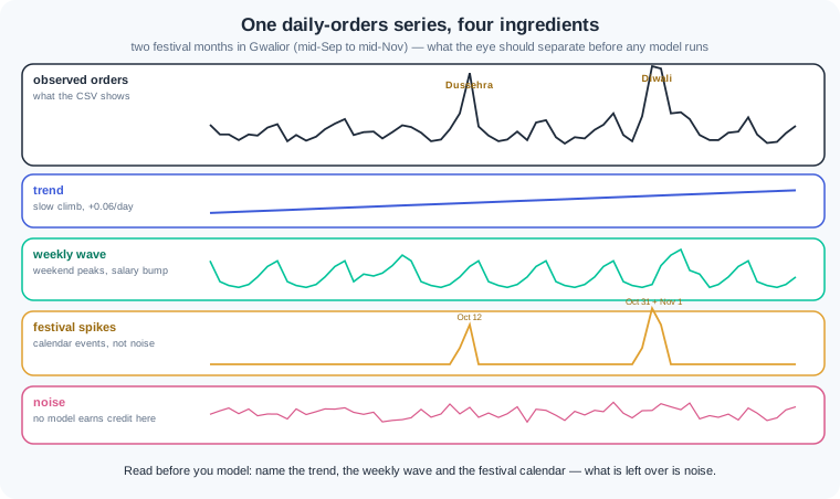
Pandas is built for this reading. Give a series a datetime index and dates become tools: slice a month by name, group by weekday, mark salary week in one line. Resampling — changing the grain of a series, like collapsing daily rows into weekly totals. Resampling also exposes a trap: a missing day is not a zero-order day. Fill gaps with zeros and you invent crashes the platform never had — the model then learns them as fact.
Before any model, run three baselines. The naive forecast copies yesterday's value forward. The seasonal-naive — copy the value from the same day one week ago — respects the weekly rhythm at zero cost. The moving average predicts the mean of the last seven days. These lazy rules embarrass fancy models often enough that professionals always score them first; a model that cannot beat last Sunday deserves no compute.
So how do the models you already know join in? Turn time into columns. A lag feature — an earlier value of the series copied into today's row, like yesterday's orders or last Monday's. Rolling-window features summarise the recent past the same way, with one iron rule: shift before rolling, so today's window ends at yesterday. Add day-of-week, salary-week and festival flags, and forecasting becomes a plain supervised table — every model from this phase applies.
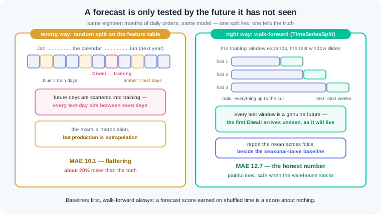
One habit from earlier modules must now be broken on purpose: the random split. The wrong way scatters future days into training, so every test day sits between days the model has seen, and the score flatters. The right way is walk-forward validation — train on everything up to a cut, test on the window after it, slide the cut forward, repeat. scikit-learn ships this as TimeSeriesSplit, an expanding window that mimics how the model will live. Report the mean MAE across windows, always beside the seasonal-naive number it must beat.
This module stays with pandas and scikit-learn on purpose. Dedicated forecasting tools exist — statsmodels for classical decomposition and ARIMA-family models, Prophet for calendar-heavy business series — and interviews expect you to name them. Reach for them when horizons stretch or series multiply into the hundreds. The habits do not change: read the series, score the baselines, walk forward.
Work inside ai-lab. One seeded world carries the whole lesson: daily orders for Swati's kirana platform, with real weekly rhythm, salary bumps and festival spikes.
Build the world. Two years of daily orders — trend, weekly lift, salary week, a festival calendar, noise:
import numpy as np
import pandas as pd

rng = np.random.default_rng(42)
days = pd.date_range("2024-07-01", "2026-06-30", freq="D")
t = np.arange(len(days))

week_lift = np.array([0, -4, -6, -3, 5, 16, 22])[days.dayofweek]
salary_lift = np.where(days.day <= 5, 12, 0)
festivals = pd.to_datetime([
    "2024-08-19", "2024-10-12", "2024-10-31", "2024-11-01",
    "2025-03-14", "2025-08-09", "2025-10-02", "2025-10-20",
    "2025-10-21", "2026-03-04",
])
on_festival = days.isin(festivals).astype(int)
on_eve = days.isin(festivals - pd.Timedelta(days=1)).astype(int)
noise = rng.normal(0, 9, len(days))

orders = np.round(110 + 0.06 * t + week_lift + salary_lift
                  + 85 * on_festival + 35 * on_eve + noise).clip(min=0)
sales = pd.Series(orders, index=days, name="orders")

print("days:", len(sales))
print(sales.loc["2025-10-18":"2025-10-22"].astype(int))
days: 730
2025-10-18    160
2025-10-19    192
2025-10-20    268
2025-10-21    209
2025-10-22    133
Freq: D, Name: orders, dtype: int64
Read the Diwali window. A normal Saturday sits near 160; the eve climbs to 192, Diwali day hits 268, and two days later life is back at 133. That 100-order swing is not noise — it is a calendar event, and the generator (like reality) wrote it in deliberately. Every trap in this lesson comes from treating dated structure like this as random.
The datetime index at work — and the gap trap. Weekday rhythm, weekly totals, then a four-day outage to show what a hole looks like:
print(sales.groupby(sales.index.dayofweek).mean().round(1))
weekly = sales.resample("W").sum()
print("first full week:", int(weekly.iloc[1]),
      "  latest full week:", int(weekly.iloc[-2]))

broken = sales.drop(sales.loc["2025-07-14":"2025-07-17"].index)
refilled = broken.asfreq("D")
print("days lost:", len(sales) - len(broken),
      "  NaN days after asfreq:", int(refilled.isna().sum()))
The weekday profile prints Monday 136.3 down to Wednesday 128.5, then up through Friday 140.0, Saturday 151.0, Sunday 155.1 — the weekly wave, measured in one line. resample("W").sum() prints first full week: 820 latest full week: 1095: weekly totals grew by a third across two years, which is the trend with the weekly wave averaged out. Then the gap drill: dropping four days and calling asfreq("D") prints days lost: 4 NaN days after asfreq: 4. Pandas restored the calendar and marked the holes NaN — the honest state. What you fill them with is a decision, and WR-083 is the story of teams who chose zero.
Three baselines before any model. Score the lazy rules on the last 28 days, exactly as a warehouse would have lived them:
test = sales.iloc[-28:]
naive = sales.shift(1).iloc[-28:]
seasonal_naive = sales.shift(7).iloc[-28:]
moving_avg = sales.shift(1).rolling(7).mean().iloc[-28:]

mae = lambda pred: (test - pred).abs().mean()
print(f"naive last-value      MAE: {mae(naive):.1f}")
print(f"seasonal-naive (t-7)  MAE: {mae(seasonal_naive):.1f}")
print(f"7-day moving average  MAE: {mae(moving_avg):.1f}")
Output: naive last-value MAE: 12.7, seasonal-naive (t-7) MAE: 10.9, 7-day moving average MAE: 12.3. Read the ranking. The naive rule keeps predicting Sunday's surge on Monday, so the weekly wave becomes its error. The moving average flattens the wave entirely — smooth, and wrong on every weekend. The seasonal-naive respects the rhythm by copying the same weekday, and at 10.9 orders it is the number to beat: any model that scores above it loses to a one-line rule from a fresher's notebook.
Time becomes a table. Lags, a shifted rolling mean, and calendar flags turn forecasting into the supervised problem you already know:
df = pd.DataFrame({"orders": sales})
df["lag_1"] = df["orders"].shift(1)
df["lag_7"] = df["orders"].shift(7)
df["lag_14"] = df["orders"].shift(14)
df["roll7_mean"] = df["orders"].shift(1).rolling(7).mean()
df["dayofweek"] = df.index.dayofweek
df["salary_week"] = (df.index.day <= 5).astype(int)
df["is_festival"] = df.index.isin(festivals).astype(int)
df["is_festival_eve"] = df.index.isin(festivals - pd.Timedelta(days=1)).astype(int)
df = df.dropna()
print("supervised rows:", len(df))
It prints supervised rows: 716 — fourteen rows fell to dropna, because lag_14 needs two weeks of history before its first honest value. Study the shape of what remains: each row now holds its own past (three lags and a rolling mean) plus its calendar (weekday, salary week, festival flags), and the target is that day's orders. Note the discipline in shift(1).rolling(7): today's rolling mean ends at yesterday. Drop the shift and today's answer leaks into today's feature — WR-084 measured what that lie costs in production.
Walk-forward, model against baseline. TimeSeriesSplit gives five expanding-window exams; the boosted model from earlier modules must beat the seasonal-naive on each genuine future:
from sklearn.ensemble import HistGradientBoostingRegressor
from sklearn.model_selection import TimeSeriesSplit
from sklearn.metrics import mean_absolute_error

feats = ["lag_1", "lag_7", "lag_14", "roll7_mean",
         "dayofweek", "salary_week", "is_festival", "is_festival_eve"]
X, y = df[feats], df["orders"]

tscv = TimeSeriesSplit(n_splits=5, test_size=56)
model_maes, base_maes = [], []
for k, (tr, te) in enumerate(tscv.split(X), 1):
    model = HistGradientBoostingRegressor(random_state=42)
    model.fit(X.iloc[tr], y.iloc[tr])
    m = mean_absolute_error(y.iloc[te], model.predict(X.iloc[te]))
    b = mean_absolute_error(y.iloc[te], X.iloc[te]["lag_7"])
    model_maes.append(m); base_maes.append(b)
    print(f"fold {k}  train {len(tr):>3} days  "
          f"model MAE {m:5.1f}   seasonal-naive MAE {b:5.1f}")
print(f"mean          model MAE {np.mean(model_maes):5.1f}   "
      f"seasonal-naive MAE {np.mean(base_maes):5.1f}")
Five folds print, training size expanding from 436 to 660 days: fold 1 reads model MAE 16.1 seasonal-naive MAE 23.5, folds 2 to 5 read 9.8 against 13.1, 9.9 against 11.6, 12.5 against 15.1 and 8.8 against 11.7, and the mean line reads model MAE 11.4 seasonal-naive MAE 15.0. Fold 1 is the story: its test window runs late September to mid-November 2025 — Dussehra and Diwali — where copying last week misses every spike and the baseline balloons to 23.5, while the model, which saw the 2024 festival season and carries festival flags, holds at 16.1. Across all five honest futures the model beats the baseline by 3.6 orders a day. That is a real win, won fairly — and now you can say exactly what it beat, and by how much.
Work inside ai-lab. Every world is seeded: where a check states a number, your number must match it exactly.
If your numbers are close but not identical, triage in a fixed order before touching your code. Everything off by a little — every value drifting in the last decimal or two — points at a library version: run pip show scikit-learn, compare it with the pinned install line from 1.2, and match the pin, because the printed numbers were produced on that version. One number wildly off while the rest agree points at stale state: restart from a fresh kernel or a fresh python and run the file top to bottom, since seeded draws only reproduce when they happen in the same order from a clean start. Only when both checks pass and the numbers still disagree should you suspect your own logic — diff your script line by line against the printed code.
Read the series before touching a model. In read_series.py, rebuild the watch block's world exactly (seed 42, dates 2024-07-01 to 2026-06-30, the same lifts, festivals and noise draw). Then measure each ingredient. (a) Print the weekday profile: mean orders per dayofweek, rounded to 1. (b) Print the mean for year one (2024-07-01 to 2025-06-30) and year two (2025-07-01 to 2026-06-30). (c) Print the mean on festival days against the mean on all other days. (d) Print the mean inside salary week (day of month 5 or lower) against the rest. Close with a five-line memo naming, with its number, each ingredient: trend, weekly seasonality, festival effect, salary effect, and the one component no model should chase. Check: the weekday profile runs from Wednesday's low of 128.5 to Sunday's high of 155.1 — a swing of 26.6 orders; year one prints 128.8 and year two prints 149.9, a climb of about 21; festival days print 230.1 against 138.1 for ordinary days — an uplift of 92 orders; salary week prints 150.0 against 137.2; your memo ties each number to its ingredient and names noise as the leftover nobody models.
The baseline gauntlet. A new city, a shorter history, and the question every forecast must answer: what does the model beat? In gauntlet.py, build daily meal-kit orders for Ujjain with np.random.default_rng(7) and pd.date_range("2025-01-01", "2026-06-30") — 546 days whose only festivals are late in the series. Draw in this exact order: week_lift from the array [0, -5, -7, -4, 6, 20, 26] indexed by dayofweek; salary_lift of 15 where day of month is 5 or lower; festivals at 2025-10-02, 2025-10-20, 2025-10-21 and 2026-03-04 with festival lift 90 and eve lift 40; noise as one rng.normal(0, 10, len(days)) call. Then orders = np.round(140 + 0.08*t + week_lift + salary_lift + 90*on_festival + 40*on_eve + noise).clip(min=0). Build the watch block's eight-feature supervised table and drop the NaN rows. Now run the gauntlet with TimeSeriesSplit(n_splits=5, test_size=56): on each fold's test window, score four forecasters by MAE — naive (the lag_1 column), seasonal-naive (lag_7), moving average (roll7_mean), and HistGradientBoostingRegressor(random_state=42) fitted on that fold's training rows. Print one honest table: a row per fold plus a mean row, four MAE columns. Below it, write a verdict paragraph: which forecaster ships, what it beats and by how much, which fold hurt everyone and why, and one fold where a baseline beat the model. Check: the table holds 532 supervised rows starting 2025-01-15; fold 1 (test late September to mid-November 2025 — the series' first festival season, which no training row contains) is the worst for everyone: naive 21.2, seasonal-naive 25.8, moving average 23.5, model 19.1; in fold 2 the seasonal-naive at 9.9 beats the model at 13.1; the mean row reads naive 16.7, seasonal-naive 15.5, moving average 16.3, model 12.7; your verdict ships the model, states it beats the best baseline by 2.8 orders a day, names the unseen festival season as fold 1's cause, and admits the fold where the lazy rule won.
Break it: the flattering random split. Take gauntlet.py's finished table and model, and evaluate them the forbidden way. In random_lie.py, split the same supervised table with train_test_split(test_size=0.25, random_state=42, shuffle=True), fit the same HistGradientBoostingRegressor(random_state=42) on the shuffled training rows, and print its test MAE beside the walk-forward mean MAE from the gauntlet. Then count how many of the table's festival-day rows the shuffled split placed into training. Close with a three-sentence confession that quantifies the lie: how many orders per day the random split hides, what that is as a percentage, and why the shuffled exam was easier — the model was quizzed on days sitting between days it had already seen, including a festival season it will never get to see in advance again. Check: the random split prints MAE 10.1 against the walk-forward 12.7 — a lie of 2.6 orders a day, about 20 percent rosier; all 4 festival rows land in training, so the "unseen festival" disaster from the gauntlet's fold 1 is invisible; your confession states both numbers and names interpolation between seen days as the flattery's source.
The gap that invented zeros. Replay WR-083 on the watch world, with the truth held in your hand. In gap_drill.py, rebuild the seed-42 world, then store the true values of 2025-07-14 to 2025-07-20 before deleting those seven rows — a one-week ingestion outage. Restore the calendar with asfreq("D") and print how many NaN days appear. Now repair the hole three ways and score each against the truth you kept: fillna(0); interpolate(method="time"); and a seasonal fill that copies each missing day from seven days earlier. Print the MAE of each repair on the lost week, then the weekly resample("W").sum() total for that week under the truth, the zero fill and the seasonal fill. Close with a three-line gap policy for your future pipelines: what a gap becomes first, how you decide between a true zero and a fill, and how a filled row stays visible. Check: the outage leaves 723 rows and asfreq prints 7 NaN days; the repairs score fillna(0) 134.9, time interpolation 9.4, seasonal fill 10.9 — the zero fill is worse by more than a factor of ten; the weekly totals print 944 for the truth, 0 for the zero fill and 990 for the seasonal fill; your policy makes gaps NaN first, demands a documented closure before any true zero, and flags filled rows in a was_filled column.
Three forecasting disasters cover most of what this lesson meets in production. Each has a War Room entry with the full diagnosis path:
- WR-082 — the festival the model never met. A demand model trained on three quiet months sailed through October blind; Diwali demand ran 40-60% over its forecast and shelves emptied, and the fix is a festival calendar as data, a manual uplift until history exists, and a humility window during flagged weeks.
- WR-083 — the resample that invented zeros. Missing days became zero-order days somewhere in a pipeline, so the model learned crashes that never happened and planners cut stock on phantom quiet days; the cure is gaps-as-NaN first, fills chosen by rule, and a flag on every reconstructed row.
- WR-084 — the rolling feature that peeked. A centred rolling mean put tomorrow inside today's features, bought a brilliant backtest and a uselessly lagging live model; shift before rolling, audit features as-of the prediction moment, and share one feature function between training and serving.
Time order is information, and a shuffled split destroys the thing a forecast must learn. Read the series first: the trend, the weekly and salary rhythm, the festival spikes, and the leftover noise. Score the three cheap baselines before any model, because a model that cannot beat last Sunday deserves no compute. Lag features and shifted rolling windows turn the series into a plain table that any model from this phase can learn. Test by walking forward through time with TimeSeriesSplit, and report honest MAE beside the copy-last-week number it must beat.
- Quick-commerce and kirana platforms forecast orders per dark store each day to stock overnight. Their festival calendars are versioned data files, and every team knows what its model beats.
- Power grid operators forecast electricity demand around the clock. Load swings with heat, weekday rhythm and festival evenings, and one point of error moves crores in generation cost.
- Banks and ATM networks forecast cash demand on the salary cycle you measured here. Stocking an ATM for the first week of the month is Swati's warehouse question with currency.
Answer these before opening the gate assessment. Each question names its type.
type=output-prediction— A series' last seven days, Monday to Sunday, read 120, 118, 115, 122, 131, 148, 155. Predict tomorrow's (Monday's) forecast under naive last-value, seasonal-naive, and 7-day moving average. Then say which rule you expect closest to the truth on this series and what its weekday profile tells you.type=debug— A teammate's demand model prints backtest MAE 4.2, but its first live month scores 9.8 and every forecast trails the series' turns by a day. The feature list includesroll7 = orders.rolling(7, center=True).mean(). Name the fault, explain why the backtest never caught it, and give the one-line repair plus the audit that proves the repair worked.type=interpretation— A walk-forward table reads: fold 1 model 19.1 baseline 25.8, fold 2 model 13.1 baseline 9.9, folds 3-5 model comfortably ahead, mean model 12.7 baseline 15.5. The fold 1 window covers the series' first festival season. Explain what fold 1 and fold 2 each reveal, and why the mean alone would hide both stories.type=scenario-judgement— An ops pipeline lost nine days to an outage, and a teammate proposesfillna(0)"since we genuinely took zero orders through the app that week". Judge the proposal, name the two separate damages zeros would cause (one to lag features, one to weekly reports), and state the repair plan you would approve instead.type=trade-off— For a single kirana store's daily forecast, compare shipping the seasonal-naive rule against shipping the boosted lag-feature model that beats it by 2.8 orders a day. Give one concrete strength and one concrete cost of each, name the operational condition under which the baseline is the right choice, and say when you would escalate to statsmodels or Prophet instead.
Explain to a friend who runs a tea stall how you would guess tomorrow's milk order. Cover why "same as last Monday" is a strong first guess (the week has a rhythm), why festival days need their own rule (the calendar, not luck), and why the only fair test of any guessing trick is pretending to forecast days that have already passed — using only what you knew the night before. Use at most 4 sentences and no word fancier than "rhythm". If your friend can say why beating "same as last Monday" is the bar any clever trick must clear, you own this module.