Coding round for AI roles
Bhaskar joined a shared screen for his first coding round in Bilaspur. Three problems, ninety minutes, one interviewer watching. He read problem one, said nothing, and started typing. Eighteen minutes later the interviewer asked what he was thinking. His code was nearly right, and it broke on an empty table. He never tested it. He solved two of the three problems and still lost the round. The note said one word: communication.
- This round is where most AI-role offers are won or lost, and it is the one you can rehearse the most cheaply. A laptop and a timer are the whole setup.
- The problems that come up for data and AI roles are not the ones most students grind. Aiming at the right three buckets saves you weeks.
- Half the marks here are for how you work, not what you produce. That half is a habit, and habits are faster to build than talent.
A coding round for an AI or data role is a mix, and the mix is not the one a product-company software round uses. Three buckets cover most of what you will meet. Data work comes first, then plain Python fluency, then a small slice of data structures and algorithms. The figure names each bucket and the spine modules that feed it.
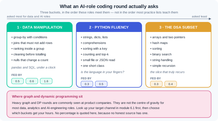
Bucket one is data manipulation, and for these roles it is the biggest one. You get a table or two and a question with conditions inside it. Group by a key and count only some rows. Join two tables without changing the row count. Clean a dirty column before you can total it.
The same bucket asks the question in SQL as often as in pandas. A window function — a SQL feature that ranks or totals rows inside a group without collapsing the group into one row — is how "top store per city" gets asked. Modules 0.5, 0.6 and 1.6 already taught these moves. What is new is doing them in eight minutes while somebody watches. That is a speed problem, not a knowledge problem.
Bucket two is Python fluency. Strings, dictionaries and lists, comprehensions, sorting with a key, counting things, reading a small file or a JSON blob, and writing one short class. Nothing here is clever. The test is whether the language is in your fingers or in your notes. If you pause to recall how sorted takes a key, that pause costs you more than the syntax.
Bucket three is the data structures and algorithms subset that truly recurs for these roles. Arrays and two pointers, hash maps, sorting, binary search, string handling, and simple recursion. Two pointers — two markers that move through a sorted list from both ends — answers pair and de-duplication questions with no extra memory. A hash map — a lookup table that finds a key in about one step, which is Python's dict — turns many slow scans into one pass.
Here is the contrast this module exists for. The wrong way is to grind three hundred graph and dynamic-programming problems because a popular list says so. Heavy graph and dynamic-programming rounds are more of a product-company pattern, and they are commonly seen there. The right way is to look up your target channel in module 6.1, then spend your hours on the buckets that channel actually asks. A student aiming at an analytics team in a bank and a student aiming at a product company should not have the same practice plan.
Complexity talk sounds academic until it costs you a job. Time complexity — how the running time grows as the input grows — is the language interviewers use for that cost. O(n) means the work doubles when the rows double. O(n squared) means the work goes up four times when the rows double. On a ten-lakh-row table that difference is hours against seconds, and the timing demo below measures it on this laptop.
That arithmetic is the same one you met in module 4.9. A nightly batch job has a window, and a job that misses the window is a failed job. So when an interviewer asks for the complexity, they are not testing your theory marks. They are asking whether you can tell in advance if your code will finish before the report is due.
Now the part that decides most rounds: the protocol. Five steps, in order, out loud. Restate the problem in your own words, state your assumptions, write the brute force, say its complexity, improve it, then test it with edge cases. A brute force — the first correct answer you can think of, however slow — is worth real marks, because a slow correct answer beats a fast blank screen.
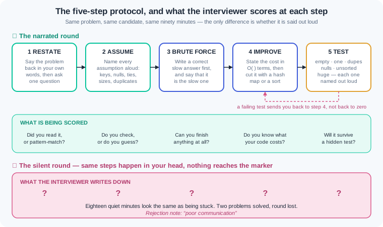
Silence is the quiet killer, and Bhaskar's round is the proof. From the other side of the screen, a thinking candidate and a stuck candidate look exactly the same. The interviewer cannot mark what they cannot hear. Say what you are trying, say why you dropped an idea, and say when you are stuck and what you would check next. Thinking aloud feels strange for about two days and then it feels normal.
Testing is the step students skip, and it is the cheapest one to add. An edge case — an input at the boundary of what your code expects — is where hidden tests live. Run the same checklist every time: empty input, one element, duplicates, nulls, unsorted order, and a huge input. Say each one out loud and say what your code does with it. That habit is worth more marks than one extra clever trick.
Online judges fail you with a message, and reading it fast is a skill. Find three things in order: which test failed, what your code gave, and what was expected. Then ask which bucket of the checklist that input belongs to, because the failing test is nearly always an edge case you skipped. A "time limit exceeded" message is different, and it means your complexity is wrong, not your logic. WR-156 walks through one of those.
One rule about model use, and it has two halves. A proctored coding round means no language model, in the same way module 6.2 treats a proctored test. Practising with a model as a tutor is a different thing, and this programme encourages it. Our stance is tutor, not generator, and it rests on verified evidence that AI-generated homework goes with worse exam scores. Ask the model to review the code you wrote, never to write the code you should have.
Six problems, run the way you should run them in the room. Every block below was executed, and the commented output at the foot of each block is what it really printed. Type each one yourself before you read the explanation under it.
Problem 1 — the pandas question under interview conditions. You have a table of UPI transactions and a store master. For each city, report the transaction count, the failed count and the failure rate, keep cities with three or more transactions, and sort by rate:
# FENCE 1 - the pandas problem, solved the way you would in the room.
import pandas as pd

txns = pd.DataFrame({
    "txn_id":   ["T1", "T2", "T3", "T4", "T5", "T6", "T7", "T8"],
    "store_id": ["S1", "S1", "S2", "S2", "S2", "S3", "S3", "S4"],
    "status":   ["SUCCESS", "FAILED", "FAILED", "SUCCESS", "FAILED",
                 "SUCCESS", None, "FAILED"],
    "amount":   [120, 80, 250, 60, 90, 150, 40, 300],
})
stores = pd.DataFrame({"store_id": ["S1", "S2", "S3", "S4"],
                       "city": ["Bilaspur", "Bilaspur", "Raipur", "Raipur"]})

# STEP 1 restate: per city, total txns, failed txns, failure rate;
#                 keep cities with 3 or more txns; sort by rate, high first.
# STEP 2 assumptions I say out loud:
#   - store_id in stores is unique (I will check, not assume)
#   - status None means "unknown", and unknown is NOT a failure
#   - "3 or more txns" counts every row, including unknown-status rows
print("master key unique?", stores["store_id"].is_unique)

# STEP 3 brute force first - a plain Python loop. O(n) but slow and wordy.
city_of = dict(zip(stores["store_id"], stores["city"]))
tally = {}
for sid, st in zip(txns["store_id"], txns["status"]):
    c = city_of[sid]
    t, f = tally.get(c, (0, 0))
    tally[c] = (t + 1, f + (1 if st == "FAILED" else 0))
print("brute force:", tally)

# STEP 4 improve - the pandas version an interviewer expects.
def city_report(txns, stores):
    d = txns.merge(stores, on="store_id", how="left", validate="many_to_one")
    d["is_failed"] = (d["status"] == "FAILED").astype(int)
    out = d.groupby("city", dropna=False).agg(
        total=("txn_id", "count"), failed=("is_failed", "sum")).reset_index()
    out["fail_rate"] = (out["failed"] / out["total"]).round(3)
    return out[out["total"] >= 3].sort_values("fail_rate", ascending=False)

print(city_report(txns, stores).to_string(index=False))

# STEP 5 complexity, said out loud: one merge on a hashed key plus one
# group-by pass. Both are about O(n) in the number of rows.

# STEP 6 TEST IT - the edge cases, before I say "done".
empty = txns.iloc[0:0]
print("empty ->", city_report(empty, stores).shape)
print("one row ->", city_report(txns.head(1), stores).shape)
allnull = txns.assign(status=None)
print("all status null ->", city_report(allnull, stores)["failed"].tolist())

# ---------- REAL OUTPUT, run on an ordinary laptop ----------
# master key unique? True
# brute force: {'Bilaspur': (5, 3), 'Raipur': (3, 1)}
#     city  total  failed  fail_rate
# Bilaspur      5       3      0.600
#   Raipur      3       1      0.333
# empty -> (0, 4)
# one row -> (0, 4)
# all status null -> [0, 0]
Read the comments as the script of what you say aloud. The uniqueness check on line one of the answer is not decoration: it is you refusing to assume, and it earns marks on its own. The brute-force dictionary loop gives {'Bilaspur': (5, 3), 'Raipur': (3, 1)}, and the pandas version must agree with it — that agreement is your own test, not the interviewer's. The three edge cases at the end each print something: an empty frame gives zero rows, a one-row frame gives zero rows because the three-transaction rule removes it, and an all-null status column gives zero failures rather than a crash.
Problem 1 again, done the two common wrong ways. Both wrong answers print a number, which is what makes them dangerous:
# FENCE 2 - the two wrong answers that pass the sample and fail the hidden test.
import pandas as pd

txns = pd.DataFrame({
    "txn_id":   ["T1", "T2", "T3", "T4", "T5", "T6", "T7", "T8"],
    "store_id": ["S1", "S1", "S2", "S2", "S2", "S3", "S3", "S4"],
    "status":   ["SUCCESS", "FAILED", "FAILED", "SUCCESS", "FAILED",
                 "SUCCESS", None, "FAILED"],
})

# WRONG 1: the master table has S2 twice (an old row and a renamed row).
dirty_master = pd.DataFrame({
    "store_id": ["S1", "S2", "S2", "S3", "S4"],
    "city": ["Bilaspur", "Bilaspur", "Bilaspur city", "Raipur", "Raipur"],
})
blown = txns.merge(dirty_master, on="store_id", how="left")
print("rows before merge:", len(txns), " rows after merge:", len(blown))
print(blown.groupby("city")["txn_id"].count().to_dict())
print("counted txns:", blown.groupby("city")["txn_id"].count().sum(), "not 8")

# WRONG 2: the master is missing S4 entirely, so city becomes NaN,
# and group-by throws NaN groups away without a word.
short_master = pd.DataFrame({"store_id": ["S1", "S2", "S3"],
                             "city": ["Bilaspur", "Bilaspur", "Raipur"]})
m = txns.merge(short_master, on="store_id", how="left")
print("null cities after merge:", int(m["city"].isna().sum()))
print("dropna default:", m.groupby("city")["txn_id"].count().sum())
print("dropna=False  :", m.groupby("city", dropna=False)["txn_id"].count().sum())

# THE GUARD that catches both, in one line each, before you say "done".
try:
    txns.merge(dirty_master, on="store_id", how="left", validate="many_to_one")
except Exception as e:
    print("validate caught it:", type(e).__name__, "-", str(e).splitlines()[0])
assert len(m) == len(txns), "merge changed the row count"
print("row-count guard passed on the good merge")

# ---------- REAL OUTPUT ----------
# rows before merge: 8  rows after merge: 11
# {'Bilaspur': 5, 'Bilaspur city': 3, 'Raipur': 3}
# counted txns: 11 not 8
# null cities after merge: 1
# dropna default: 7
# dropna=False  : 8
# validate caught it: MergeError - Merge keys are not unique in right dataset;
#                     not a many-to-one merge
# row-count guard passed on the good merge
Eight transactions went into the first merge and eleven came out, because a duplicate key in the master multiplies rows. Nothing warned you, and the per-city counts now total 11 instead of 8 — this is WR-014 wearing an interview costume. The second failure is quieter still: one store is missing from the master, so its city is null, and group-by drops null groups by default, so the total silently falls from 8 to 7. The two guards at the bottom cost one line each. Say them out loud in the room: "I will validate the merge as many-to-one, and I will assert the row count did not change."
Problem 2 — the same question in SQL, plus the window-function shape. SQLite ships with Python, so this runs on any laptop with no install:
# FENCE 3 - the SQL problem. sqlite3 ships with Python, so this runs offline.
import sqlite3

db = sqlite3.connect(":memory:")
db.executescript("""
CREATE TABLE txns (txn_id TEXT, store_id TEXT, status TEXT, amount INTEGER);
CREATE TABLE stores (store_id TEXT, city TEXT);
INSERT INTO txns VALUES
 ('T1','S1','SUCCESS',120), ('T2','S1','FAILED', 80), ('T3','S2','FAILED',250),
 ('T4','S2','SUCCESS', 60), ('T5','S2','FAILED', 90), ('T6','S3','SUCCESS',150),
 ('T7','S3', NULL,      40), ('T8','S4','FAILED',300);
INSERT INTO stores VALUES ('S1','Bilaspur'),('S2','Bilaspur'),
                          ('S3','Raipur'),('S4','Raipur');
""")

# Q1: same question as the pandas one. Conditional counting inside GROUP BY.
q1 = """
SELECT s.city,
       COUNT(*)                                        AS total,
       SUM(CASE WHEN t.status = 'FAILED' THEN 1 ELSE 0 END) AS failed,
       ROUND(1.0 * SUM(CASE WHEN t.status = 'FAILED' THEN 1 ELSE 0 END)
             / COUNT(*), 3)                            AS fail_rate
FROM txns t
JOIN stores s ON s.store_id = t.store_id
GROUP BY s.city
HAVING COUNT(*) >= 3
ORDER BY fail_rate DESC;
"""
for row in db.execute(q1):
    print(row)

# Q2: the window-function shape. Highest-value txn per city, ties kept.
q2 = """
SELECT city, txn_id, amount FROM (
  SELECT s.city, t.txn_id, t.amount,
         RANK() OVER (PARTITION BY s.city ORDER BY t.amount DESC) AS rk
  FROM txns t JOIN stores s ON s.store_id = t.store_id)
WHERE rk = 1 ORDER BY city;
"""
print("--- top txn per city ---")
for row in db.execute(q2):
    print(row)

# THE TRAP an interviewer plants here: COUNT(status) is not COUNT(*).
print("--- count trap ---")
print(db.execute("SELECT COUNT(*), COUNT(status) FROM txns").fetchone())

# ---------- REAL OUTPUT ----------
# ('Bilaspur', 5, 3, 0.6)
# ('Raipur', 3, 1, 0.333)
# --- top txn per city ---
# ('Bilaspur', 'T3', 250)
# ('Raipur', 'T8', 300)
# --- count trap ---
# (8, 7)
The first query prints the same two rows as the pandas answer, which is the point: one question, two languages, one result. SUM(CASE WHEN ... THEN 1 ELSE 0 END) is the conditional-count pattern, and it is worth memorising because it answers a whole family of questions. The second query is the window-function shape; RANK() OVER (PARTITION BY ...) numbers rows inside each city without collapsing them, so "top per group" needs no self-join. The last line is the trap that catches careless candidates: COUNT(*) is 8 and COUNT(status) is 7, because counting a column skips nulls. Say that difference out loud before the interviewer has to ask.
Problem 3 — the Python-fluency question, brute force then improved. Count error codes in a log and return the top three, ties broken by code:
# FENCE 4 - the Python-fluency problem, brute force first, then improved.
from collections import Counter

logs = [
    "10:04:11 ERROR 429 /predict", "10:04:12 INFO 200 /predict",
    "10:04:13 ERROR 500 /score",   "10:04:15 ERROR 429 /predict",
    "10:04:18 ERROR 503 /score",   "10:04:19 ERROR 500 /predict",
    "10:04:21 INFO 200 /health",   "10:04:25 ERROR 429 /score",
]

# RESTATE: from these lines, return the 3 most common ERROR codes,
#          highest count first, and break ties by the code, low first.
# ASSUME (said out loud): only lines marked ERROR count; a code is the
#          third field; fewer than 3 distinct codes returns what exists.

def top_errors_brute(lines, k=3):          # the version I write first
    codes = [l.split()[2] for l in lines if l.split()[1] == "ERROR"]
    pairs = []
    for c in set(codes):                   # for each distinct code ...
        pairs.append((c, codes.count(c)))  # ... scan the whole list again
    pairs.sort(key=lambda p: (-p[1], p[0]))
    return pairs[:k]

def top_errors(lines, k=3):                # the version I improve to
    codes = Counter(l.split()[2] for l in lines if l.split()[1] == "ERROR")
    return sorted(codes.items(), key=lambda p: (-p[1], p[0]))[:k]

print("brute   :", top_errors_brute(logs))
print("improved:", top_errors(logs))
# COMPLEXITY out loud: brute is O(n x k) because .count() rescans per code.
# Improved is one pass, O(n), plus a sort of the distinct codes, O(k log k).

# TEST IT - the checklist, run before I say "done".
print("empty      :", top_errors([]))
print("one line   :", top_errors(["09:00:00 ERROR 404 /x"]))
print("no errors  :", top_errors(["09:00:00 INFO 200 /x"]))
print("all same   :", top_errors(["09:00:00 ERROR 500 /x"] * 4))
tie = ["09:00:00 ERROR 503 /x", "09:00:01 ERROR 500 /x"]
print("tie order  :", top_errors(tie), "-> 500 before 503")
print("k bigger   :", top_errors(tie, k=9))
print("agree?     :", top_errors_brute(logs) == top_errors(logs))

# ---------- REAL OUTPUT ----------
# brute   : [('429', 3), ('500', 2), ('503', 1)]
# improved: [('429', 3), ('500', 2), ('503', 1)]
# empty      : []
# one line   : [('404', 1)]
# no errors  : []
# all same   : [('500', 4)]
# tie order  : [('500', 1), ('503', 1)] -> 500 before 503
# k bigger   : [('500', 1), ('503', 1)]
# agree?     : True
The two versions print the same list, and that agreement is the whole reason to write the slow one first. The sort key (-count, code) is the move to keep: a minus sign sorts numbers high-to-low while the second field still sorts low-to-high, so ties come out in a fixed order. Say the complexity in plain words — the brute version rescans the list once per distinct code, and the improved version reads it once. Six of the eight printed lines are edge cases, and the last one is a self-check that costs a single line.
Problem 4 — the DSA-subset question, run through the full protocol. Find two amounts that add to a target. This is the hash-map and two-pointer pattern in one problem:
# FENCE 5 - the DSA-subset problem, run through the full five-step protocol.

# RESTATE: given refund amounts and a target, find two DIFFERENT positions
#          whose amounts add up to the target. Return one pair or None.
# ASSUME  : integers, may repeat, may be negative; any valid pair is fine;
#           one element cannot pair with itself.

def pair_brute(nums, target):              # STEP 3: brute force, O(n^2)
    for i in range(len(nums)):
        for j in range(i + 1, len(nums)):
            if nums[i] + nums[j] == target:
                return (i, j)
    return None

def pair_hash(nums, target):               # STEP 4a: hash map, O(n) time
    seen = {}                              # value -> its position
    for i, v in enumerate(nums):
        if target - v in seen:
            return (seen[target - v], i)
        seen[v] = i
    return None

def pair_two_pointer(sorted_nums, target): # STEP 4b: two pointers, sorted input
    lo, hi = 0, len(sorted_nums) - 1
    while lo < hi:
        s = sorted_nums[lo] + sorted_nums[hi]
        if s == target: return (lo, hi)
        if s < target:  lo += 1
        else:           hi -= 1
    return None

amounts = [250, 80, 120, 300, 60]
print("brute  :", pair_brute(amounts, 380))
print("hash   :", pair_hash(amounts, 380))
print("2-ptr  :", pair_two_pointer(sorted(amounts), 380), "on", sorted(amounts))
# COMPLEXITY out loud: brute O(n^2) time, O(1) extra memory. Hash map O(n)
# time and O(n) memory. Two pointers O(n) time and O(1) memory, but it needs
# sorted input, so sorting first makes the whole job O(n log n).

# STEP 5 TEST IT - empty, one, duplicates, none, negatives, unsorted.
cases = [([], 10), ([5], 10), ([5, 5], 10), ([1, 2, 3], 100),
         ([-40, 90, 40, 0], 0), ([300, 60, 250], 310)]
for nums, t in cases:
    b, h = pair_brute(nums, t), pair_hash(nums, t)
    print(f"{str(nums):>20} target {t:>4} -> brute {str(b):>8} hash {str(h):>8}",
          "| same:", (b is None) == (h is None))
print("duplicate trap: [5,5] must return (0, 1), never (0, 0)")

# ---------- REAL OUTPUT ----------
# brute  : (1, 3)
# hash   : (1, 3)
# 2-ptr  : (1, 4) on [60, 80, 120, 250, 300]
#                   [] target   10 -> brute     None hash     None | same: True
#                  [5] target   10 -> brute     None hash     None | same: True
#               [5, 5] target   10 -> brute   (0, 1) hash   (0, 1) | same: True
#            [1, 2, 3] target  100 -> brute     None hash     None | same: True
#     [-40, 90, 40, 0] target    0 -> brute   (0, 2) hash   (0, 2) | same: True
#       [300, 60, 250] target  310 -> brute   (1, 2) hash   (1, 2) | same: True
# duplicate trap: [5,5] must return (0, 1), never (0, 0)
Notice the two-pointer answer is (1, 4) while the other two give (1, 3), and both are correct — the positions refer to different orderings, which is exactly the kind of assumption you must state before you code. The [5, 5] case is the duplicate trap: writing if target - v in seen before storing v is what stops an element pairing with itself. The empty and one-element cases return None rather than crashing, because both loops never start. Saying the memory cost alongside the time cost is a small line that separates a prepared candidate from a rehearsed one.
The timing demo — what O(n squared) costs on a real table. This is the module 4.9 arithmetic, measured on an ordinary laptop:
# FENCE 6 - what O(n^2) and O(n) mean on a 10-lakh-row job. Measured, not told.
import time

def has_dup_quadratic(ids):        # O(n^2): compare every pair
    for i in range(len(ids)):
        for j in range(i + 1, len(ids)):
            if ids[i] == ids[j]:
                return True
    return False

def has_dup_linear(ids):           # O(n): one pass, a set remembers
    seen = set()
    for x in ids:
        if x in seen:
            return True
        seen.add(x)
    return False

def timed(fn, data):
    t = time.perf_counter(); fn(data); return time.perf_counter() - t

print(f"{'rows':>9} {'O(n^2) sec':>11} {'O(n) sec':>10} {'ratio':>8}")
base = None
for n in (2000, 4000, 8000):
    ids = list(range(n))                       # worst case: no duplicate
    q, l = timed(has_dup_quadratic, ids), timed(has_dup_linear, ids)
    if base is None: base = (n, q)
    print(f"{n:>9} {q:>11.3f} {l:>10.5f} {q / l:>8.0f}x")

big = list(range(1_000_000))
lin_big = timed(has_dup_linear, big)
n0, q0 = base
predicted = q0 * (1_000_000 / n0) ** 2         # quadratic scaling rule
print(f"{1000000:>9} {predicted:>11.0f} {lin_big:>10.5f} (predicted, not run)")
print(f"predicted O(n^2) at 10 lakh rows = {predicted / 3600:.1f} hours")
print(f"measured  O(n)   at 10 lakh rows = {lin_big:.3f} seconds")

# TIE TO 4.9: a nightly batch job has a window. Say the window is 30 minutes.
window = 30 * 60
print(f"fits in a {window // 60}-min window? "
      f"O(n^2): {predicted <= window}   O(n): {lin_big <= window}")

# ---------- REAL OUTPUT, one ordinary laptop, one run ----------
#      rows  O(n^2) sec   O(n) sec    ratio
#      2000       0.026    0.00004      615x
#      4000       0.097    0.00007     1398x
#      8000       0.399    0.00016     2500x
#   1000000        6398    0.01983 (predicted, not run)
# predicted O(n^2) at 10 lakh rows = 1.8 hours
# measured  O(n)   at 10 lakh rows = 0.020 seconds
# fits in a 30-min window? O(n^2): False   O(n): True
Your numbers will differ from these, and the shape will not. Look at the quadratic column: doubling the rows from 2000 to 4000 took 0.026 to 0.097 seconds, which is about four times, and doubling again gave 0.399, four times over. That is what "quadratic" means with your own stopwatch, and it is why the predicted figure at ten lakh rows is 1.8 hours against a measured 0.020 seconds for the one-pass version. A nightly job with a thirty-minute window fails on one and finishes on the other, which is the module 4.9 point in a single line. When a judge says "time limit exceeded", this table is what happened to you.
Work in a folder called coding-round with three files that grow all week: problems.md for every problem you attempt, protocol-card.md for the five steps and the edge-case checklist, and scores.csv for your self-scoring. Score the protocol separately from correctness, always, because they fail separately in a real round.
Build the protocol card and the edge-case checklist, then run them once. Write protocol-card.md by hand: the five steps in order, and under each step two sentences you will actually say out loud, in your own words. Then write the edge-case checklist as six named cases — empty, one element, duplicates, nulls, unsorted, huge — and for each one write what it usually breaks and one sentence you say when you test it. Now take the pandas problem from fence 1, close this page, and redo it from scratch with a twelve-minute timer, speaking every line of the card as you go. Record nothing yet; the aim is to hear yourself use the card once. Check: the card holds five steps and six edge cases with your own sentences under each, not copied ones; your solution agrees with a brute-force loop you wrote yourself; you tested at least four of the six edge cases and wrote down what each one printed; you can state the complexity of your answer in one sentence without looking; and you noted the one step of the five you skipped under time pressure, because there always is one.
The timed problem set: ten problems, ninety minutes, three buckets. Assemble ten problems before you start the clock, from free public practice sets or from your own data: four data-manipulation problems (two pandas, two SQL, at least one needing a join that must not change the row count and one needing a per-group ranking), three Python-fluency problems (one counting or sorting with a key, one string or dictionary task, one small class or JSON read), and three from the recurring subset (one two pointers, one hash map, one binary search or simple recursion). Set a nine-minute cap per problem and obey it by the clock. Score every problem out of five for correctness and out of five for protocol, where the protocol marks are one each for restating, stating assumptions, writing a brute force, saying the complexity, and testing edge cases aloud. Check: ten problems and the marking scheme are saved before the timer starts, not after; scores.csv holds twenty numbers with a one-line reason for every protocol mark you did not award; your bucket totals are computed separately so you can see which bucket is weakest; you name the single protocol step you lost the most marks on across all ten; and you write one sentence stating whether correctness or protocol cost you more, with the totals behind it.
Record yourself thinking aloud, then mark your own tape. Pick two problems you have not seen, one from data manipulation and one from the recurring subset. Record audio or screen video while you solve each one in twenty minutes, speaking continuously through all five steps. Then play both recordings back with a notebook and log three things against the timestamp: every silence longer than twenty seconds, every assumption you acted on without saying it, and every edge case you never tested. Write a one-line replacement sentence for each silence — the words you should have said at that moment. Check: two recordings exist with their lengths noted; the silence log gives a timestamp and a replacement sentence for every gap over twenty seconds; you counted your unstated assumptions and can name the riskiest one; you list the untested edge cases and say which one a hidden test would most likely use; and you re-record the first two minutes of one problem using your replacement sentences, and note whether the longest silence shrank.
Complexity first, then measure, then fix a failing judge test. Take five problems where a slow answer is possible: duplicate detection, top-k counting, pair sum, a group-by over a large table, and a substring search. For each one, before writing any code, write down your predicted complexity for both a brute-force answer and an improved answer. Then write both, and time both at three input sizes using time.perf_counter, exactly as fence 6 does. Build a table of measured seconds and check whether the growth matches your prediction, then extrapolate each brute force to ten lakh rows and say whether it fits a thirty-minute batch window. Finish by taking any one of your brute-force answers, feeding it an input large enough that it would time out, and writing the two-line diagnosis you would give an interviewer. Check: predictions are written before the code, with timestamps or file history proving the order; five timing tables exist with three sizes each and the measured ratios computed; every prediction is marked right or wrong against the measurement, with a sentence on any that surprised you; the ten-lakh extrapolation is shown as arithmetic and turned into a yes-or-no answer on the batch window; and your diagnosis names the complexity, the input size at which it breaks, and the specific change that fixes it.
Three failures cover most first-season coding rounds. Each has a War Room entry with the full diagnosis path:
- WR-154 — the silent candidate. A student solved the problem correctly in his head, said nothing for eighteen minutes, and was rejected for poor communication; the fix is the narration protocol with the exact sentences to say at each of the five steps.
- WR-155 — the untested edge case. Code that passed the visible example failed a hidden test on an empty input and a duplicate key; the fix is running the six-case checklist out loud before the word "done" is ever said.
- WR-156 — the nested loop that timed out. A correct answer hit the judge's time limit because it compared every pair of rows; the fix is a complexity estimate before coding, plus the measured timing intuition from fence 6.
A coding round for AI roles is mostly data work, then Python fluency, then a small recurring slice of data structures and algorithms. Practise by channel using the module 6.1 map, because heavy graph and dynamic-programming rounds are more of a product-company pattern. Run the same five steps out loud every time: restate, state assumptions, write the brute force, say the complexity, improve, and test. Silence reads as being stuck, so narrate what you try and what you drop, and run the six-case edge checklist before you say you are done. Estimate complexity before you write code, because the gap between one pass and every pair is hours against seconds on a ten-lakh-row table.
- Analytics and reporting teams at Indian banks and fintechs screen with exactly the fence 1 and fence 3 questions. A join that changes the row count is a real money error in a UPI settlement report, not a puzzle.
- Data engineering roles in logistics and retail ask the complexity question for a reason. A nightly batch over a parcel table must finish inside its window, and the fence 6 table is the arithmetic behind that promise.
- AI and machine learning teams in GCCs use the same protocol in daily work. Restating a task, naming assumptions and testing edge cases is how a feature pipeline gets reviewed, so the round is a sample of the job.
Answer these before opening the gate assessment. Each question names its kind.
type=output-prediction— A candidate merges 8 transaction rows against a store master where one store code appears twice, then printslen(result)and a per-city count. Predict what the row count becomes and what the per-city counts total, and name the one argument that would have raised an error instead.type=debug— A submission passes the visible example and fails the hidden tests withIndexError: list index out of range. The function starts withlo, hi = 0, len(nums) - 1and immediately readsnums[lo]. Name the failing input, explain the mechanism in one sentence, and give the one-line fix.type=interpretation— A timing run gives 0.026 seconds at 2,000 rows, 0.097 at 4,000 and 0.399 at 8,000. State what growth pattern this is and how you know from these three numbers alone, then estimate the time at 10 lakh rows and say what it means for a thirty-minute batch window.type=scenario-judgement— Fifteen minutes are left, and you have a working answer that compares every pair of rows. The interviewer has not commented. Give your ruling on what you do next and the exact first sentence you say, and justify it against the five-step protocol.type=trade-off— For a pair-sum question, compare a hash-map answer against a sort-then-two-pointers answer. Give one concrete gain and one concrete cost of each, then say which you would offer first when the interviewer says the input is already sorted and memory is tight.
Explain to a friend in a non-technical degree why a coding interview marks how you work and not only whether the code runs. Describe the five steps in the order you would do them, using an everyday task such as counting bills in a kirana shop, and say why staying quiet while you think loses marks. Then tell your friend the one check you always run before saying you are finished. Use at most 4 sentences and no word your friend would need to look up. If your friend can name the five steps and the one final check, you own this module.